Publications

The Research Data Centres Information and Technical Bulletin

Weighted estimation and bootstrap variance estimation for analyzing survey data: How to implement in selected software

Archived Content

Information identified as archived is provided for reference, research or recordkeeping purposes. It is not subject to the Government of Canada Web Standards and has not been altered or updated since it was archived. Please "contact us" to request a format other than those available.

By Christian Gagné, Georgia Roberts & Leslie-Anne Keown

Introduction

This document is for analysts/researchers who are considering doing research with data from a survey where both survey weights and bootstrap weights are provided in the data files.

This document gives directions, for some selected software packages, about how to get started in using survey weights and bootstrap weights for an analysis of survey data.

The software covered in this document are:

SUDAAN 10
Svy commands in STATA 12
WesVar 5.1
Survey procedures in SAS 9.2
Bootvar 3.2 for SAS

Details about other software packages that can do appropriate weighted estimation and also accommodate survey bootstrap weights for variance estimation will be added to this document in the future.

We first provide a checklist of a number of items that an analyst should consider after identifying his major research questions and after doing preliminary investigation of his potential data source(s). Some of the questions in the checklist are specific to the particular analytical problem being undertaken while others relate to the particular software being considered. In order for the checklist to be comprehensive, it may contain questions that do not apply to all analyses.

We next describe an example of analysis from a particular survey. This example will be used to illustrate the different software. More examples could be added to a later edition of this document.

Finally, we give brief directions for obtaining survey-weighted estimates, bootstrap variance estimates (and other desired error quantities) and some typical test statistics for each software package in turn. While these directions are provided just for the chosen examples, there will be information about the range of weighted and bootstrapped analyses that can be carried out by each software package.

In the appendix we provide information on other topics that have been identified by researchers and analysts who are analyzing survey data. One such topic is a discussion of the normalizing of weights. Other topics will be added over time. The References section includes publications that are referred to in the document as well as a number of books containing explanations about why and how the survey design should be accounted for in analysis.

For researchers to get the most from this document, we advise that they begin by reviewing the checklists below, followed by a reading of the example and the completion of the problem-specific checklist for this example. Then the researchers could move to the sections of the document related to the specific software that they are considering for carrying out their analyses; there they can read about the software-specific checklist for the example and implementation of the software for it.

Checklist for analysis using weighting and bootstrap variance estimation

Problem-specific checklist

Have you clearly spelled out what questions you want to answer in your analysis?
Has a suitable analytic sample with appropriate variables been identified?
Have you clearly identified what types of analysis will be required? (e.g., types of descriptive statistics, types of model)
Have you concluded that weighted estimates and bootstrap variance estimates (errors) are appropriate for the analyses? (While, for most analyses, weighted estimation and design‑based variance estimation through bootstrapping can be recommended, there are situations where this may not be the best approach for an analysis.)
Have you determined what additional tests and statistics will be needed?
Have you consulted the survey user guide (and other documentation) and determined the following:
1. Sample size release guidelines
2. Any cautions on appropriate analytical methods
3. Appropriate survey weight variable (e.g., household or person weight; longitudinal or cross-sectional weight) and corresponding bootstrap weight variables
4. Whether bootstrap weight variables are mean bootstraps, and, if so, the number of replicate samples that were used to generate each mean bootstrap weight (which is needed for a bootstrap weight adjustment)? [Appendix C of the BootVar User Guide provides this information for a large number of surveys.]

Software-specific checklist

Have you determined that the required weighted estimates, bootstrap variance estimate (errors) and tests/statistics are available with the software being used?
If the specific tests and statistics desired are not available, is it possible to write a post‑estimation program to calculate them, in the software being used?
Is it possible, in the software, to restrict the sample or to remove out-of-sample observations from the full survey data file?
If the survey weight, the bootstrap weights and the analysis variables are not in the same file, do you know how to merge the different sources in the software being used? (This is assuming that the software being used requires that all this information be in the same file.)
While doing your analysis, have you checked the output from the software to determine:
1. that the correct sample size was used
2. that the correct weight variable was used
3. that the entire set of bootstrap weights was used
4. that the mean bootstrap adjustment was correctly implemented (if needed)
5. whether there were any bootstrap samples for which estimates could not be made?

GSS example: Using data from General Social Survey Cycle 22

The GSS program, established in 1985, conducts telephone surveys across the 10 provinces. The GSS is recognized for its regular collection of cross-sectional data that allows for trend analysis, and its capacity to test and develop new concepts that address emerging issues. The GSS program gathers data on social subjects in order to monitor changes in the living conditions and well-being of Canadians over time and to provide immediate information on specific social policy issues of current or emerging interest.

Cycle 22 is the second cycle of the GSS to collect data on social engagement and social networks. The first was Cycle 17 – Social Engagement in 2003.

The target population for Cycle 22 of the GSS included all persons 15 years of age and older in Canada in 2008, excluding:

Residents of the Yukon, Northwest Territories, and Nunavut;
Full-time residents of institutions.

Computer assisted telephone interviewing (CATI) was used to collect data for GSS-22. For sampling, the target population was divided into geographic strata. Households were selected using a Random Digit Dialling method (RDD), which randomly generates a list of phone numbers used to reach households. Once contact is made with a chosen household, a survey respondent aged 15 or over is selected to participate in the survey. Respondents were interviewed in the official language of their choice and interviews by proxy were not permitted. Data for Cycle 22 of the GSS were collected in 5 waves, from February to November 2008.

Problem-specific checklist, example for GSS

One aspect of social engagement, which is the special focus of GSS 22, is civic participation. One topic covered by the survey, as part of civic participation, was political engagement. The researcher is interested in whether or not people are voting and whether some particular factors seem to be related to their decision to vote or not.

1. Have you clearly spelled out what questions you want to answer in your analysis?

There are two questions of interest:

How did people respond when asked whether they voted in the last federal election? What proportion of the population is estimated to have made each of the different types of responses?
Given that a person is aged 20 to 64 and that the person is willing to reveal whether or not he voted in the last federal election, is the probability of voting related to sex, age group (20-29, 30-44, 45-64), and rural/urban location? Once sex and urban/rural location have been taken into account, is age group still significantly related to the probability of voting?

2. Has a suitable analytic sample with appropriate variables been identified?

GSS 22 seems to contain the variables needed for the analyses, and appears to be adequate for the particular population of interest to the researcher. The target population for GSS 22 is a little wider than the one of interest, with respect to age range (since it covers those aged 15+ and we are only interested in those aged 20-64), but could be a little more limited than desired in the type of people covered (since it does not cover residents of the Yukon, Northwest Territories, and Nunavut or full-time residents of institutions.). The researcher would need to decide whether these limitations are of importance to him. (The confidential microdata file for GSS 22 is certainly another option as a data source but would have the same limitations with respect to target population.)

Either the Public Use Microdata File (PUMF) or the confidential data file for GSS 22 could be used for the analysis. We will illustrate this example using the PUMF, since this file is more accessible to allow testing of various software in places other than in an RDC. The analytical variables (and their values) on the PUMF that have been identified for the analysis are the following:

Table 1a-d

It can be seen that the variable on the data file related to whether or not a person voted in the last federal election, PER_Q110, has possible values other than just “Yes” and “No”. The researcher will need to decide how to handle these. The AGEGR5 variable provides the age of respondents by age group categories, and categories 03 to 11 cover the full age range of interest and allow the creation of the age groups of interest. The urban/rural indicator variable, LUC_RST, has a category for urban, another for rural, and then a third category for Prince Edward Island; again, the researcher will need to decide how to handle this variable in his analysis. For the example here, we decided to include observations from PEI in the Rural and Small Town category. It frequently makes sense to recode problem variables, based on the decisions made, rather than working with the original variables.

3. Have you clearly identified what types of analysis will be required?

For question 1(a) above, a procedure that estimates proportions of a population with specified characteristics will be required. It will also be necessary to obtain estimates of variability of these estimated proportions, such as estimates of variances, standard errors or coefficients of variation.

For question 1(b) above, a procedure that carries out logistic regression on the target subpopulation (i.e., those aged 20 to 64 who revealed whether or not they voted) would seem appropriate. The dependent variable could be the logit of the probability of voting while the independent variables could be sex (with “female” as the reference category), age (two variables with “45-64” as the reference category) and urban/rural (with “urban” as the reference category and Prince Edward Island considered part of the rural category). We will also need to examine the variability of the estimated model coefficients, as well as carry out particular tests about the model coefficients.

4. Have you concluded that weighted estimates and bootstrap variance estimates (errors) are appropriate for the analysis?

Yes. Weighted estimates and bootstrap variance estimates are appropriate for both estimates of proportions and for fitting and testing of a logistic regression model.

5. Have you determined what additional tests and statistics will be needed?

Generally, for a logistic model, a researcher wants to test for the significance of each coefficient in the model; such tests are usually part of the default output from a logistic regression. However, the researcher has specified that he also wants to test whether age contributes significantly to the model, after controlling for sex and urban/rural location. Worded differently, a test is required for whether the coefficients on both of the age variables in the underlying model are significantly different from 0, given that sex and urban/rural location are in the model.

6. Have you consulted the survey user guide (and other documentation) and determined the following:

Sample size release guidelines
The User Guide for GSS 22 states: “Users should determine the number of records on the microdata file which contribute to the calculation of a given estimate. This number should be at least 15 in the case of persons. When the number of contributors to the weighted estimate is less than this, the weighted estimate should generally not be released regardless of the value of the Approximate Coefficient of Variation. If it is, it should be with great caution and the insufficient number of contributors associated with the estimate should be prominently noted.”
Guidelines regarding coefficients of variation (CV) must also be taken into account. See the user guide for GSS 22.
Any cautions on appropriate analytical methods
Users are encouraged in the GSS 22 user guide to use weighted estimates and estimate variances using the bootstrap weights.
Appropriate survey weight variable and corresponding bootstrap weight variables.
On the PUMF file for GSS 22, the person weight variable and corresponding bootstrap weights are named respectively “wght_per” and “wtbs_001” - “wtbs_500”. (There is also a household weight variable, but no corresponding bootstrap weights are provided. Thus, further guidance from the data provider would be required before doing any analyses with the household weight.)
Whether bootstrap weight variables are mean bootstraps, and, if so, the number of replicates in each mean bootstrap weight (needed for a bootstrap weight adjustment)
The bootstrap weights were generated using the “Mean Bootstrap” methodology. Each mean bootstrap weight is generated from 25 regular bootstrap samples. [See Phillips (2004) for a brief description of mean bootstrap weights.]

SUDAAN 10

Overview

SUDAAN is a statistical software package for the analysis of correlated data, including correlated data encountered in complex sample surveys. SUDAAN 10 was released in August 2008 and is comprised of nine analytic procedures as well as two pre-analytic procedures. It provides estimates that account for complex design features of a study such as unequal weighting, stratification, multistage and cluster designs, repeated measures, general cluster correlation and multiply-imputed analysis variables.

SUDAAN 10 offers three variance estimation methods – Taylor series, jackknife and BRR. The BRR option can be used with user-specified bootstrap weights in order to obtain bootstrap variance estimates (as explained in Phillips (2004)).

The SAS-callable version of SUDAAN 10 is the one used for the material in this document. In this version, calls to SUDAAN procedures are embedded in a SAS program, which means that the data management strengths of SAS can be combined with the survey analysis strengths of SUDAAN.

The following table points out the main types of analysis that can be carried out by SUDAAN 10, using weighted estimation and bootstrap variance estimation. The particular SUDAAN procedure(s) for obtaining these analyses are also provided.

Table 2
Main types of analysis in SUDAAN 10

Details about each procedure can be found in the SUDAAN Language Manual and SUDAAN Example Manual, which are accessible online when the software is installed.

Software-specific checklist example for GSS

1. Have you determined the following:

The required weighted estimates and bootstrap variance estimates (errors) are available with the software being used?
SUDAAN can compute the required weighted estimates and bootstrap variance estimates for the types of analysis needed for the example, and for many other types of analysis as shown in the table above. However, SUDAAN does not produce estimates of CV’s that may be required for some quantities in order to check for compliance with release guidelines.
As described in Phillips (2004), choosing the BRR option in SUDAAN for variance estimation and providing the bootstrap weight variables will result in bootstrap variance estimates. Phillips (2004) also indicates how choice of the BRR option with a Fay adjustment will correctly calculate mean bootstrap variance estimates.
Thus, to invoke weighted estimation and bootstrap variance estimation for any SUDAAN procedure, include the following:
- In the PROC statement, include the DESIGN=BRR option
- Include a WEIGHT statement to identify the survey weight variable to be used for weighted estimation
- Include a REPWEIGHT statement to indicate the names of the bootstrap weight variables on the data file. If the bootstrap weight variables are mean bootstrap variables, add the ADJFAY option to the REPWEIGHT statement. The ADJFAY value simply consists of the number of bootstrap samples used to produce each mean bootstrap variable. (The ADJFAY option is omitted if you have ‘regular’ bootstrap weights.)
For the particular GSS example, where the weight variable is wght_per, the 500 mean bootstrap weight variables are wtbs_001 to wtbs_500 and each is formed from 25 bootstrap samples, every SUDAAN procedure used would contain the following:

PROC procedurename data=SAS_datafile_name design=BRR; WEIGHT wght_per; REPWEIGHT wtbs_001-wtbs_500 / ADJFAY=25; +Other statements required by the procedure
Note: The SUDAAN documentation indicates that a WEIGHT statement is optional. However, if the WEIGHT statement is omitted, the mean of the bootstrap weights is used as the weight variable. This changes the values of both the weighted estimates and of the bootstrap variance estimates, and is thus not advised if consistency with usual estimates is desired.
The required tests and statistics are available with the software being used?
For the GSS example we want to test that each individual logistic model coefficient is 0, and also that the coefficients on the two age dummy variables are simultaneously 0.
The results of such tests are part of the default output from PROC rlogist, as demonstrated later. However, it is also possible to request other statistics to test the same thing or to test more complex relationships among the coefficients of the model, as part of the call to PROC rlogist.

2. If the specific tests desired are not available, is it possible to write a post-estimation program to calculate them, in the software being used?

For this particular example, any desired tests can be obtained from SUDAAN. However, in order to provide some outlook on the analyses where this may not be the case, the following information is provided.

It is not possible to write a post-estimation program in SUDAAN to calculate tests that are not included in SUDAAN. However, since the SUDAAN procedures are embedded within a SAS program, it is generally possible to output a wide range of the SUDAAN results into a SAS program to calculate what is required. Through the use of an OUTPUT statement, a variety of estimates can be output in a ready-to-use format. For example, the full variance‑covariance matrix of a set of estimates can be output; this matrix (rather than just variance estimates) is needed for many test statistics. One particular situation where it would be useful to output estimated quantities and then to use these quantities in a SAS program is for the computation of CV’s, which SUDAAN does not provide. (Note that the CV of an estimate is simply the ratio of the standard error of the estimate to the estimate itself.)

3. Is it possible, in the software, to restrict the sample or to remove out-of-sample observations from the full survey data file?

An analysis in SUDAAN can be restricted to the sample with particular characteristics (often called the sample in a particular subpopulation) by the use of a SUBPOPN statement in a SUDAAN procedure. The SUBPOPN statement must be included in every SUDAAN procedure where the restricted sample is required.

Alternatively, it is also straightforward to restrict the sample or remove out-of-sample observations from the full survey data file by writing the code for a DATA step of a SAS program before the call to a SUDAAN procedure. This produces a smaller data file that can then be used as the input data file for all SUDAAN procedures where the restricted sample is required.

The merging of the different sources would need to be done in SAS before the SUDAAN procedures are used. SUDAAN, however, does not require that the bootstrap weights be in the same data file as the survey weight and the analysis variables. The SUDAAN Language Manual gives directions about how to specify a different file for bootstrap weights.

5. While doing your analysis, have you checked the output from the software to determine:

that the correct sample size was used
that the correct weight variable was used
that the entire set of bootstrap weights were used
that the mean bootstrap adjustment was correctly implemented (if needed)
whether there are any bootstrap samples for which estimates could not be made?

The default output from a SUDAAN procedure gives the number of observations read and the number of observations used in the analysis carried out by the procedure. It also provides weighted counts of both of those quantities.
The default output from a SUDAAN procedure gives the name of the survey weight variable used.
The default output from a SUDAAN procedure lists the names of all bootstrap weight variables that were used.
It can be determined whether the correct mean bootstrap adjustment was made by seeing that the output statement “Multiplier associated with Replicate weights” contains the number of standard bootstrap samples that were combined to produce each mean bootstrap. In the case of GSS 22, this value should be 25.
If there are any bootstrap samples for which estimates could not be made, these are identified in the SUDAAN output. This did not occur in the GSS Example.

SAS/SUDAAN program and output example for GSS

Program

/* PIECE 1 */ options linesize=80; libname pumfl '\\SASD6\Sasd-Dssea-Public\DATA\GSS\DLI\CYCLE22\C22MDFSasAndCode-EngFr';

data c22pumf; set pumfl.c22pumf; run;

/* PIECE 2 */ /*Preliminary descriptive analysis*/ proc crosstab data= c22pumf design=brr; weight wght_per; repwgt wtbs_001- wtbs_500 / ADJFAY=25; class Per_Q110 /nofreq; tables Per_Q110; setenv colwidth=20 decwidth=4; print nsum=”sampsize” wsum=”popsize” rowper serow lowrow uprow; run;

/* PIECE 3 */ /*Recode variables and pick subpopulation sample*/ data c22pumfn; set pumfl.c22pumf; /*Subpopulation of voters aged 20 to 64*/ if agegr5 ge 03 and agegr5 le 11; if Per_Q110 =1 or Per_Q110 =2;

/*Recode of the Urban variable*/ if LUC_RST=1 then Urban=1; else Urban=0;

/*Recode of age variable in 3 categories*/ if agegr5 le 04 then age = 1; else if agegr5 le 07 then age =2; else if agegr5 le 11 then age =3;

/*Recode of the voted variable*/ if Per_Q110 =1 then Vote =1; else Vote =0; run;

/* PIECE 4 */ proc crosstab data= c22pumfn design=brr; weight wght_per; repwgt wtbs_001- wtbs_500 / ADJFAY=25; class Vote /nofreq; tables Vote; setenv colwidth=20 decwidth=4; print nsum=”sampsize” wsum=”popsize” rowper serow lowrow uprow; run;

/* PIECE 5 */ proc rlogist data=c22pumfn design=BRR; weight wght_per; repwgt wtbs_001- wtbs_500 / ADJFAY=25; class sex age Urban; model Vote = sex age Urban ; run;

Discussion of program and output:

PIECE 1

This piece of the program is SAS programming, where the initial PUMF SAS dataset is specified. After the execution of the data step, the SAS log (not shown) indicates that the dataset c22pumf contains 20401 records. This piece of the program does not produce any output.

PIECE 2

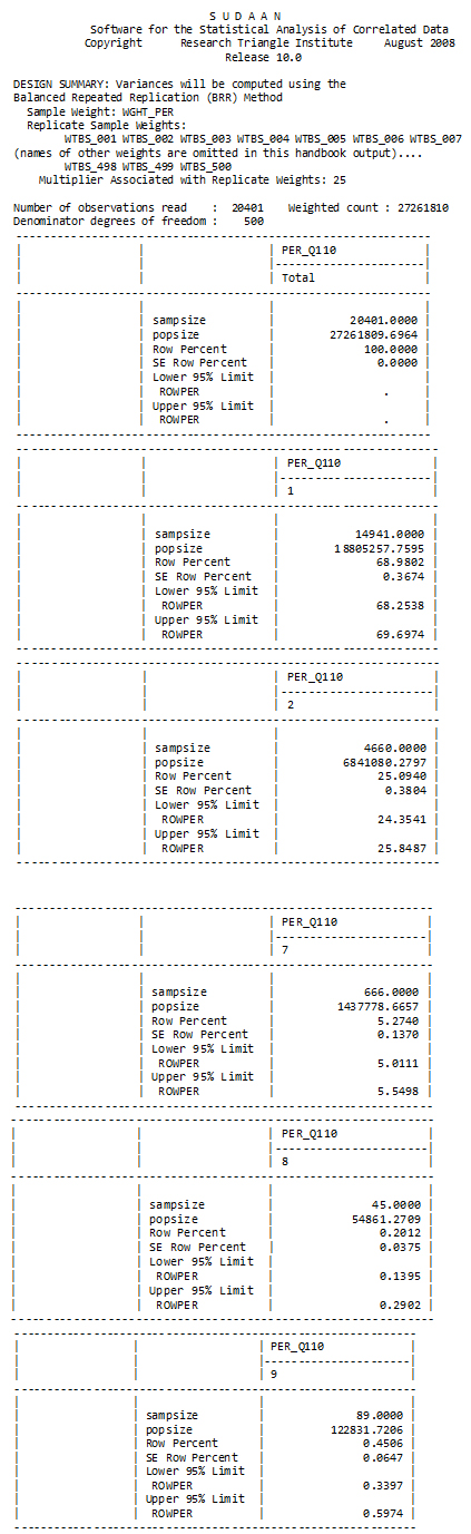
This piece of the program is a call to SUDAAN PROC CROSSTAB for obtaining estimates of the proportions of the full population that made the different types of responses to the question about voting in the last federal election. This allows a preliminary inspection of the variable Per_Q110.

As for all calls to a SUDAAN procedure, the output provides the names of the weight variable and bootstrap weight variables, the method of variance estimation used, the sample size and the estimated population size.

In order to limit the CROSSTAB output to the quantities of interest to the researcher, a PRINT statement has been used. As well as the estimated proportions and their standard errors, the sample size and estimated population size and 95% confidence limits were requested. It should be noted that SUDAAN does not provide estimates of CV’s.

As can be seen from the output, 94 % (i.e., 68.98+25.09=94.07) of the population targeted by GSS 22 is estimated to have responded either yes (=1) or no (=2) to the question on voting in the last federal election. The remainder of the population did not give a yes or no answer for a variety of reasons (values of 7, 8, or 9 for Per_Q110).

PROC CROSSTAB by default calculates the asymmetric confidence intervals for proportions using logistic transformation. If PROC DESCRIPT is used instead to calculate the proportion of a particular case involving an average, symmetrical confidence intervals are produced and are based on the assumption of a normal approximate distribution for the ratio of the proportion over its standard deviation.

Figure 1
SUDAAN output for PER_Q110 variable

Description of Figure 1 SUDAAN output for PER_Q110 variable

PIECE 3

This part of the program is a data step in SAS. In it, sample observations in the subpopulation of interest are chosen (i.e., sample observations for people aged 20 to 64 and responding “yes” or “no” to the question about voting). Then, some of the variables are recoded in order to match the categories required for the logistic regression. Here are the details of the recodes done:

Table 3
Recode of variables

After the execution of the data step, the SAS log (not shown) indicates that the new data set c22pumfn contains 14813 records. This data step does not produce any output.

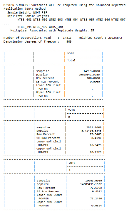
PIECE 4

This part of the program is a call to PROC CROSSTAB in SUDAAN, to obtain estimates of the percentage of the people aged 20-64 who said “yes” and the percentage who said “no” to the voting question, given that they gave one of these two answers to the question. Note that the new variable VOTE is being used, with the restricted sample. It would have been possible, instead, to have used the full data set but restrict to the subpopulation of interest by including a SUBPOPN statement in PROC CROSSTAB.

Figure 2
SUDAAN design summary and VOTE variable output

Description of Figure 2 SUDAAN design summary and VOTE variable output

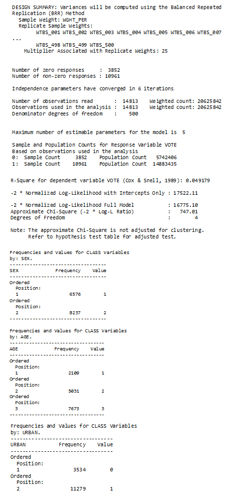
PIECE 5

This part of the program is the fitting of the logistic model to the restricted sample through a call to PROC RLOGIST in SUDAAN. The procedure is modeling the logit of the probability that VOTE=1 in the restricted sample. Note that all the information about the weight, the bootstrap weights, etc. has to be included in the call to the procedure.

Note that the default output provides information about the three variables SEX, AGE, and URBAN that are identified as being categorical in a CLASS statement. By default, the highest value of each variable will be the reference category when the program creates dummy variables. It is possible, instead, to declare what values you wish to choose as reference categories through the use of a REFLEVEL option as described in the user guide.

Figure 3
SUDAAN design summary and variables SEX, AGE, and URBAN output

Description of Figure 3 SUDAAN design summary and variables SEX, AGE, and URBAN output

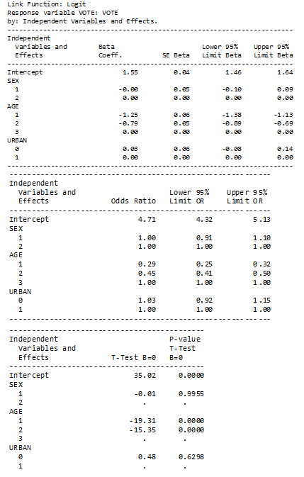
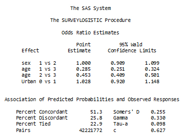
The fitted model is presented in two forms in two different tables – the first where the fitted coefficients are shown and the other where the coefficients are expressed as odds ratios. A third table presents results of t-tests on each individual coefficient.

Figure 4
SUDAAN Logit model on dependent variable VOTE

Description of Figure 4 SUDAAN Logit model on dependent variable VOTE

The table below, which is part of the default output, presents the results of tests on whether each variable contributes significantly to the model, after inclusion of the other variables. This table thus allows us to assess whether the age variable (with 2 degrees of freedom) contributes significantly to the model, given that sex and urban/rural location are already controlled. This was one of the questions of interest to the researcher. An alternative approach to testing the same hypothesis would be through the use of CONTRAST or EFFECT statements in the call to PROC RLOGIST.

Figure 5
SUDAAN regression output

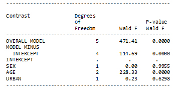
Description of Figure 5 SUDAAN regression output

STATA 12

Overview

Stata 12 release includes several features designed to work specifically with Statistics Canada bootstrap weights. Stata uses the addition of a prefix (svy) to many commands, which adapts them to working with the survey design that is set in a program statement (svyset). Stata can be operated either using syntax (program statements) in the form of a ‘do’ file or through pull‑down menus. All examples provided in this document use syntax statements.

Stata 12 offers a full suite of design-based variance estimation options with the svy commands – Taylor series, jackknife, BRR, and bootstrap. The bootstrap option can be used with user-specified survey bootstrap weights, such as those provided with many Statistics Canada surveys, in order to obtain bootstrap variance estimates. The approach to using earlier versions of Stata for obtaining bootstrap variance estimates is described in the Appendix 2.

The following table points out some of the common types of analysis that can be carried out by the svy commands in Stata 12, where weighted estimates and bootstrap variance estimates are produced. There are numerous other analytic techniques available through svy commands. A full list can be found in the appendix A1 of this document, or by consulting the Survey Data manual, the help procedure and the PDF documentation in Stata, by utilizing the FAQ or statalist archives on the Stata website, or by contacting Stata support.

Table 4
Some common analyses with svy commands in STATA 12

In addition to the svy commands, many Stata 12 commands accept survey weights in a pweight statement. Since these commands do not make use of the bootstrap weights, design‑based bootstrap variance estimation is not carried out. More discussion of this topic is included in Appendix 4 in the section on normalizing weights.

Software-specific checklist example for GSS

1. Have you determined the following:

That the required weighted estimates and bootstrap variance estimates (errors) are available with the software being used?
Stata can compute the required weighted estimates and bootstrap variance estimates for the types of analysis for the example, and for many other types of analysis as shown in the table above and in the Appendix. Basically, to produce analytical results that incorporate the survey design through the survey weight and bootstrap weights the following is required:
1. Issue a svyset command with the following specifications:
  1. pweight set to appropriate survey weight variable
  2. Bootstrap weights identified with the bsrweight option
  3. Type of variance estimation set to bootstrap with the vce option
  4. Degrees of freedom set to the default (number of bootstrap weights) or in the case of some surveys, to a smaller appropriate value. [A good approximation to degrees of freedom is the number of psu’s containing sample in the population being analyzed minus the number of strata containing sample. However, these quantities are frequently not known by the researcher. In most cases, using the number of bootstrap weights instead of this approximation will have negligible impact on results.]
  5. Mean square error option set using the mse option. (This option calculates the bootstrap variance as the average of the squared differences between bootstrap estimates and the full-sample estimate. If this option is not selected, the bootstrap variance is computed as the average of the squared differences between the bootstrap estimates and the average of the bootstrap estimates.)
  6. The mean bootstrap adjustment set, if needed, with the bsn option, which should have the value of the number of bootstrap samples used to produce each mean bootstrap weight.
2. For the particular GSS example, the survey weight variable is wght_per, the 500 mean bootstrap weight variables are wtbs_001 to wtbs_500 and each is formed from 25 bootstrap samples : Your svyset command will appear as follows:
  svyset [pweight=wght_per], bsrweight(wtbs_001- wtbs_500) bsn(25) vce(bootstrap) dof(500) mse
3. After the svyset command, Stata will produce weighted and bootstrapped estimates every time you use the svy prefix in front of a command – e.g.,. svy: mean
Have you determined that other required tests and statistics are available with the software being used?
For the GSS example, testing whether each individual coefficient of the underlying logistic model is significantly different from 0 is obtained within the default model output. Testing whether age has remained significant after controlling for sex and urban/rural location requires a joint test of the two age coefficients using the test syntax, this can be obtained through a post-estimation command.
Other post-estimation tests and procedures are available in Stata. In order to ascertain whether these tests are appropriate for results from a particular svy command, consult the user guide or Stata support directly.

2. If the specific tests and statistics desired are not available, is it possible to write a post-estimation program to calculate them, in the software being used?

Stata can implement user-written programs. In addition, Stata does provide the ability to download programs written by others to accomplish certain tasks. For details on these possibilities see the Programming and MATA guides available through Stata or online. Stata also provides full access to almost all estimates, matrices etc. that can then be used to conduct post-estimation tests in user-written programs in Stata. It is, however, the responsibility of the researcher to determine whether down-loaded programs or user-written programs are correct and are using the appropriate weighted and bootstrapped estimates in their calculations.

3. Is it possible, in the software, to restrict the sample or to remove out-of-sample observations from the full survey data file?

Sample restrictions can be done through if statements in commands, by keeping or dropping records using keep or drop commands, or by using subpopulation options within survey commands. In the GSS example, two keep commands were used to restrict the sample to appropriate observations.

The survey weight, bootstrap weights and analysis variables must appear in the same file in Stata. This can be accomplished using a one-to-one merge in Stata.

5. While doing your analysis, have you checked the output from the software to determine

that the correct sample size was used
that the correct weight variable was used
that the entire set of bootstrap weights were used
that the mean bootstrap adjustment was correctly implemented (if needed)
whether there are any bootstrap samples for which estimates could not be made?

The default output from a Stata procedure gives the number of observations read and the number of observations used in the analysis carried out by the procedure. It also provides weighted counts of both of those quantities.
The default output from the svyset command procedure in Stata gives the name of the survey weight variable used.
The default output from the svyset procedure in Stata lists the names of all bootstrap weight variables that were used. Carefully check this statement to make sure that all bootstrap weights were used. In the syntax shown here the assumption is made that all the bootstrap weights are contiguous in the file. Another way to specify the weights would be to use a wildcard (i.e. wtbs_*)
The output from the svyset procedure in Stata shows whether the mean bootstrap adjustment was applied.
If there are any bootstrap samples for which estimates could not be made, these are identified in the Stata output.

Stata program and output example for GSS

Do-File syntax

*open log file log using "F:\GSS22\pumf\example.log", replace

*open data file use "F:\GSS22\pumf\c22pumf_eng.dta", clear

*restrict sample by age keep if agegr5 >2 keep if agegr5 <12

*Recode per_q110 into new variable vote where 1=yes and 2=no 7,8,9=missing (.) recode per_q110 (1=1) (2=0) (7/9=.), gen (vote) label define vote 1 "yes" 0 "no", modify label values vote vote

*recode variable agegr5into age with 3 categories recode agegr5 (1/2=.) (3/4=1) (5/7=2) (8/11=3), gen (age) label define age 1"20 to 29 years" 2"30 to 44 years" 3 "45 to 64 years", modify label values age age

*recode luc_rst into urban recode luc_rst (1=1) (2/3=0), gen (urban) label define urban 0 "rural " 1 "urban", modify label values urban urban

*set up the survey design information for use with the svy pefix svyset [pweight=wght_per], bsrweight(wtbs_001- wtbs_500) bsn(25) vce(bootstrap) dof(500) mse

*frequency table with bootstrapped for each variable to check basic descriptives and recodes svy:tab per_q110, obs count se cv format(%14.4g) svy:tab vote, obs count se cv format(%14.4g) svy:tab vote, obs se cv format(%14.4g) svy:tab age, obs count se cv format(%14.4g) svy:tab age, obs se cv format(%14.4g) svy:tab urban, obs count se cv format(%14.4g) svy:tab urban, obs se cv format(%14.4g) svy:tab sex, obs count se cv format(%14.4g) svy:tab sex, obs se cv format(%14.4g)

*crosstabs of age and urban with vote with tests svy:tab vote age, col obs se ci cv format(%14.4g) svy:tab vote urban, col obs se ci cv format(%14.4g)

*logistic regression svy:logit vote ib2.sex ib3.age ib1.urban svy:logistic vote ib3.age ib1.urban ib2.sex test 1.age 2.age

Stata Output

These initial commands open the file, restrict the sample to the age range of interest, and recode the variables to contain the categories desired.

. *open data file . use "F:\GSS22\pumf\c22pumf_eng.dta", clear . *restrict sample by age . keep if agegr5 >2 (1057 observations deleted)

. keep if agegr5 <12 (4421 observations deleted)

. *Recode per_q110 into new variable vote where 1=yes and 2=no 7,8,9=missing (.) . recode per_q110 (1=1) (2=0) (7/9=.), gen (vote) (3962 differences between per_q110 and vote) . label define vote 1 "yes" 0 "no", modify . label values vote vote . *recode variable agegr5into age with 3 categories . recode agegr5 (1/2=.) (3/4=1) (5/7=2) (8/11=3), gen (age) (14923 differences between agegr5 and age) . label define age 1"20 to 29 years" 2"30 to 44 years" 3 "45 to 64 years", modify . label values age age . *recode luc_rst into urban . recode luc_rst (1=1) (2/3=0), gen (urban) (3559 differences between luc_rst and urban) . label define urban 0 "rural " 1 "urban", modify . label values urban urban

The svyset command below tells Stata that we have a probability weight (wght_per) to use in the calculation of estimates and a set of bootstrap weights to use in design-based variance estimation. It also tells Stata about the adjustment needed for the mean bootstrap (bsn=25). In addition, we are telling Stata to use the mean square error formula in variance estimation calculations. The output shows that all this was done.

. *set up the survey design information for use with the svy prefix . svyset [pweight=wght_per], bsrweight(wtbs_001- wtbs_500) bsn(25) vce(bootstrap) dof(500) mse

pweight: wght_per VCE: bootstrap MSE: on bsrweight: wtbs_001 wtbs_002 wtbs_003 wtbs_004 wtbs_005 wtbs_006 wtbs_007 wtbs_008 wtbs_009 wtbs_010 wtbs_011 wtbs_012 wtbs_013 wtbs_014 wtbs_015 wtbs_016 wtbs_017 wtbs_018 …(output omitted) wtbs_496 wtbs_497 wtbs_498 wtbs_499 wtbs_500 bsn: 25 Design df: 500 Single unit: missing Strata 1: <one> SU 1: <observations> FPC 1: <zero>

This first section allows us to see our number of observations, weighted counts and weighted percentages with CV’s for each variable in our analysis. Only the output for the dependent variable (vote) is shown. The number of observations decreases from 14,923 (for Per_q110) to 14,813 (for VOTE) because the observations with a missing value for VOTE are excluded from the estimate.

Figure 6
STATA bootstrapping output for PER_Q110 and VOTE variables

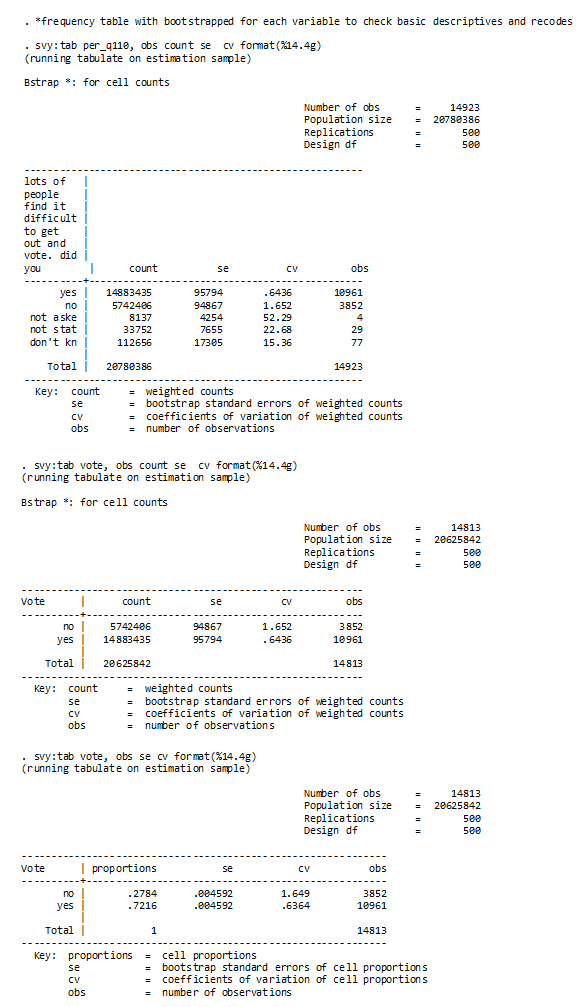
Description of Figure 6 STATA bootstrapping output for PER_Q110 and VOTE variables

Next, we look at cross-tabulations of our variable of interest (VOTE) and each covariate. Only the cross-tabulation between VOTE and AGE is shown. In each cell of each table, we can see an estimate of the proportion, the standard deviation for the proportion, the coefficient of variation, the confidence interval, and the unweighted counts. There is also a test of independence at the bottom of each table. The confidence intervals are asymmetric because they are calculated using logit transformation.

Figure 7
STATA crosstab output for the variables VOTE and AGE

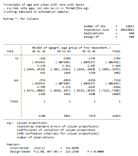
Description of Figure 7 STATA crosstab output for the variables VOTE and AGE

Two model outputs are shown below. They differ only in that one (svy: logit) shows coefficients and the other (svy: logistic) shows odds ratios. Note the use of the Survey prefix (svy) in front of the logit or logistic command. The t-tests for the coefficients or odds ratios are directly beside the estimates. The test following the fitting of the logistic model tests that the two dummy variables for age are having a significant impact on the model, after gender and urban/rural location are controlled.

Figure 8
STATA Logit model and T-tests

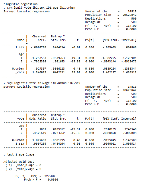
Description of Figure 8 STATA Logit model and T-tests

WesVar 5.1

Overview

WesVar is a software package produced by the Westat organization. A recent version of the package is free for download at http://www.westat.com/statistical_software/WesVar/index.cfm.

WesVar carries out various analyses of survey data using exclusively replication methods for variance estimation. One of the methods offered is BRR with a Fay adjustment, which, as explained in Phillips (2004), can be used to get bootstrap variance estimates if the bootstrap weight variables are provided by the researcher. In WesVar, the variance estimation method is specified when creating a new WesVar data file. The resulting file is then used to define workbooks where table and regression requests are carried out.

The following table points out the main types of analysis that can be carried out by WesVar 5.1, using weighted estimation and bootstrap variance estimation. The locations in the software for obtaining these analyses are also indicated.

Table 5
Main types of analysis in WesVar 5.1

Clearly-written instructions for using WesVar are provided in the User’s Guide, which can also be downloaded free of charge from http://www.westat.com/statistical_software/WesVar/index.cfm.

WesVar is a standalone program. Since it is capable of importing a wide variety of file formats, it can be readily used by researchers who have data files in such formats as SPSS or SAS data sets. The user can also output the results from the whole workbook or only one section in one or many tab-delimited text files.

WesVar has a visual interface. Thus, researchers who prefer drop-down menus for doing analysis should be comfortable with using WesVar.

Software-specific checklist example for GSS

1. Have you determined the following:

The required weighted estimates and bootstrap variance estimates (errors) are available with the software being used?
WesVar can compute the required weighted estimates and bootstrap variance estimates for the types of analysis for the example, and for many other types of analysis as shown in the table above. Selecting the bootstrap weight variables and the BRR method at the creation of the data file stage will result in correct bootstrap variance estimates, if the bootstrap weights are ‘regular’ bootstrap weights. If the bootstrap weight variables are mean bootstraps, the Fay method needs to be chosen, along with the specification of a Fay adjustment value in order to correctly calculate mean bootstrap variance estimates.
Have you determined that the required tests/statistics are available with the software being used?
For the GSS example we want to test that each individual model coefficient in the logistic regression is 0, and also that the coefficients on the two age dummy variables are simultaneously 0. The results of such tests are part of the default output from the Estimated Coefficients Tab in the Regression output page, as demonstrated later. However, it is also possible to request other statistics to test the same thing or to test more complex relationships among the coefficients of the model.

2. If the specific tests desired are not available, is it possible to write a post-estimation program to calculate them, in the software being used?

You cannot write a post-estimation program in WesVar. However, you may be able to export the required quantities from the WesVar output and then create a program in some other software, depending on what tests are desired.

3. Is it possible, in the software, to restrict the sample or to remove out-of-sample observations from the full survey data file?

When creating the WesVar Data set, the Subset Population button can be used to restrict the sample to a given subpopulation.

The merging of the different sources would have to be done in another software package before WesVar is used. WesVar requires that the bootstrap weights be in the same data file as the survey weight and the analysis variables.

5. While doing your analysis, have you checked the output from the software to determine

that the correct sample size was used
that the correct weight variable was used
that the entire set of bootstrap weights were used
that the mean bootstrap adjustment was correctly implemented (if needed)
whether there are any bootstrap samples for which estimates could not be made?

The Request output indicates the number of observations read and it provides a weighted estimate of the population size represented by the observations.
The Request output gives the name of the survey weight variable used.
The Request output lists the bootstrap weights variables that were used.
It can be determined whether the correct mean bootstrap adjustment was made by seeing that the output statement “Fay’s Factor” contains the mean bootstrap adjustment. In the case of GSS 22, this value should 0.8, since it should equal $1 - C^{\frac{1}{2}}$ , where C is the number, 25, of bootstrap samples used to produce each mean bootstrap weight variable.
The Replicate Coefficient box can be checked in the Auxiliary Output Files part of the Output Control Option in the Regression Request Tab. This produces a file that contains all the regression coefficients for each bootstrap replicate. If estimation cannot be done on a given replicate, this file will allow its identification.

Demonstration of WesVar, example for GSS

Creating a WesVar data file

WesVar can accept many file types to start with, such as data files from Stata, SAS, and SPSS. In this example, a SAS file was used to create the WesVar data file. To create a WesVar data file with mean bootstrap weights:

Move the replicate weight variables (i.e., wtbs-001 to wtbs_500) to the Replicates box.
Move the survey weight variable (i.e., wght_per) to the Full sample box.
For the mean bootstrap, specify the Method as Fay and specify Fay_K=.8.
Move any analysis variables to the Variables box and, optionally, a unique identifier variable to the ID box. For this example, RECID is a unique record identifier.
Save the file.

Figure 9
WESVAR file creation

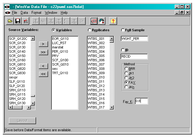
Description of Figure 9 WESVAR file creation

Creating a workbook

As stated in the user guide, “In addition to a WesVar data file, you must create a workbook. A workbook is a way to organize analyses for one project or data set. Within a workbook you can define and run Table Requests and Regression Requests, and open, view and print their output. A workbook can contain multiple Table or Regression Requests.”

As seen below, the WesVar Workbook screen is divided into two parts, with the right panel allowing you to define and change the analysis requests and with the left panel showing the workbook tree.

Figure 10
WESVAR workbook screen

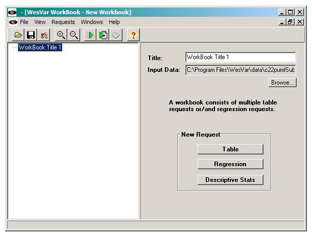
Description of Figure 10 WESVAR workbook screen

Estimation of the proportions of the population having each of the possible responses to the question on voting

To set up this analysis, the “Table” button, as seen in the screen above, is selected under “New Request”.

Next is a screen where the details of the table request are chosen. For this analysis, the variable PER_Q110 is selected, since this is the variable indicating the response to the voting question. Since the researcher is interested in the percentage of people with each value of PER_Q110, the percent box is checked, as shown below.

Figure 11
WESVAR PER_Q110 variable table request

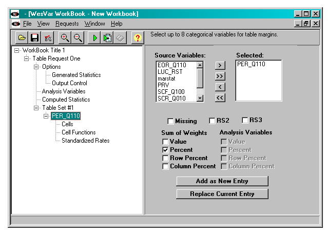
Description of Figure 11 WESVAR PER_Q110 variable table request

After all selections are made, press “Add as New Entry”, then use the “Run Selected Request” button. The output, displayed below, can be accessed with the “View Output” button.

Figure 12
WESVAR workbook output

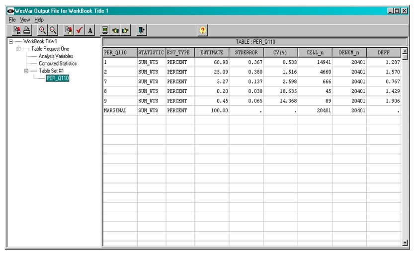
Description of Figure 12 WESVAR workbook output

Choosing a Subpopulation

The subpopulation of interest is made up of people aged 20 to 64 who are willing to reveal whether or not they voted in the last federal election (and the sample in that subpopulation are those aged 20 to 64 who had a value of 1 or 2 for the PER_Q110 variable) .

The Subset Population button is accessed through the Data File window. The subpop string to be input in this window is the following:

(AGEGR5 >= 03 and AGEGR5 <= 11) and (PER_Q110=1 or PER_Q110=2)

Figure 13
WESVAR subpopulation

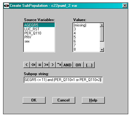
Description of Figure 13 WESVAR subpopulation

Recoding of variables

Recoding can be done to create new variables or to change values of variables. The recode button is the second to last on the right on the Data File window.

In the window below, a 0/1 variable called “Urban” is created from the LUC_RST variable. In “Urban”, rural observations and observations from PEI both are given a value of 0.

Figure 14
WESVAR recode URBAN variable

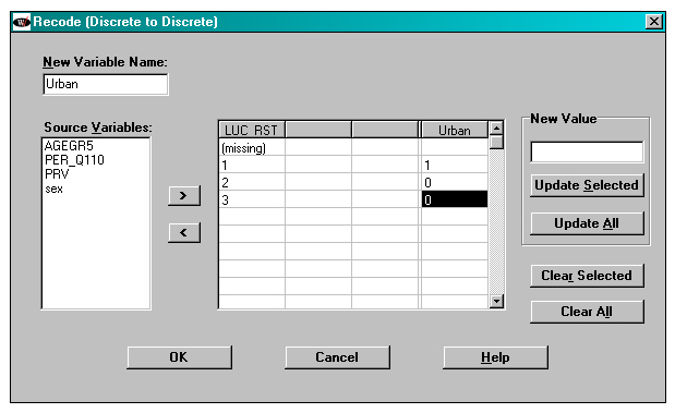
Description of Figure 14 WESVAR recode URBAN variable

In the window below, a 0/1 variable called “Vote” is created from PER_Q110. In the sample in the subpopulation, PER_Q110 just takes on values 1 and 2.

Figure 15
WESVAR recode VOTE variable

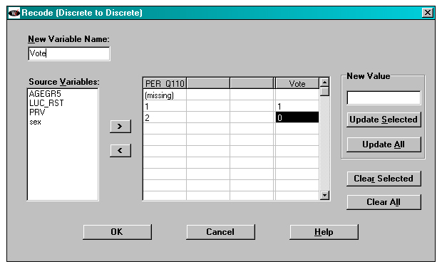
Description of Figure 15 WESVAR recode VOTE variable

The “age” variable, created from the AGEGR5 variable, has 3 categories: 1, 2, and 3 for people aged 20-29, 30-44, and 45-64, respectively. See below.

Figure 16
WESVAR recode AGE variable

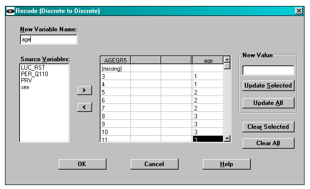
Description of Figure 16 WESVAR recode AGE variable

Clicking the “ok” button in the screen below will write new variables to the data file.

Figure 17
WESVAR pending recodes

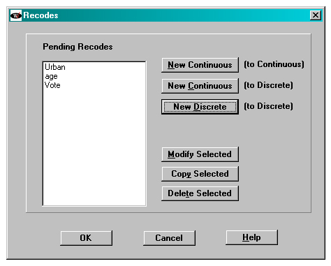
Description of Figure 17 WESVAR pending recodes

Analysis of the VOTE variable

It is now of interest to estimate the proportion of people who answered yes to the voting question and the proportion that answered no, given that they are in the subpopulation of interest. To do this, a new Request is created in the workbook using the table button. Then the Vote variable is selected from the source variables. The Add as New Entry button has to be pressed to create this specific Table request.

Figure 18
WESVAR VOTE variable table request

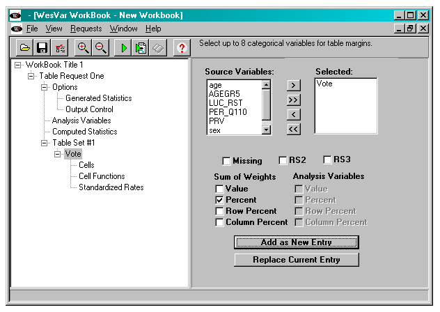
Description of Figure 18 WESVAR VOTE variable table request

The output from this request can be seen below.

Figure 19
WESVAR table request output

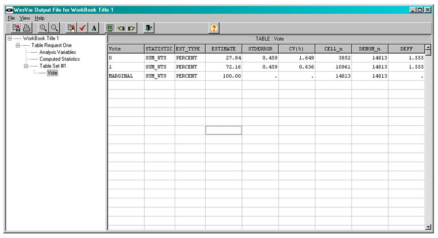
Description of Figure 19 WESVAR table request output

Logistic regression

Logistic regression is used to model the probability of voting in the last federal election as a function of sex, age and whether one lives in the city or not. The model is to be fit to the sample in the subpopulation of interest. After having selected the “Regression” button in the Workbook page, select “Logistic” in the Model Type from the Option page as shown below.

Figure 20
WESVAR Logistic regression

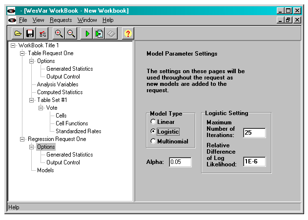
Description of Figure 20 WESVAR Logistic regression

Next, in the Regression Model Panel, choose dependent and independent variables by moving them from the Class Variables and Source Variables lists. (Any variable with less than 256 response categories will appear in the Class Variables list, along with its number of levels, as well as in the Source Variables list.) Here the Class Variables age[3], sex[2] and Urban[2] are selected to be put in the independent variable box, which means that WesVar will then create the appropriate number of 0/1 dummy variables in the model for these variables. The dependent variable, Vote, must be chosen from the Source Variables list. See below.

Figure 21
WESVAR regression model panel

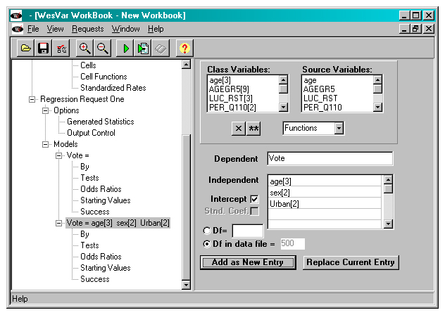
Description of Figure 21 WESVAR regression model panel

The event being modeled in a logistic regression is often referred to as “success”. For our particular example, “success” is saying “yes” to the question about whether a person voted in the last federal election. In order to make sure that we model the probability of voting, rather than the probability of not voting, we choose “1” as the source value in the Success tab of the workbook tree. (Recall that Vote=1 if a person said that they voted and Vote=0 if they said that they did not vote.) If no Success value is specified, the default value is the smaller of the two values of the dependent variable, which would mean that, for a 0/1 dependent variable, the default is to define 0 as “success”.

Figure 22
WESVAR Logistic regression

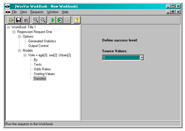
Description of Figure 22 WESVAR Logistic regression

After the logistic model request is submitted, a variety of output can be viewed through the clicking of the appropriate node in the left panel of the screen. Below can be seen the estimated model coefficients, along with estimated standard errors and the results of standard tests of whether each underlying coefficient is 0.

Figure 23
WESVAR Logistic regression output

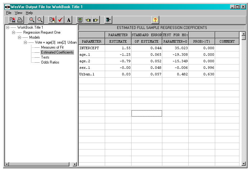
Description of Figure 23 WESVAR Logistic regression output

The panel below shows the fitted model in the form of odds ratios, along with a confidence interval on each one.

Figure 24
WESVAR fitted model, odds ratios

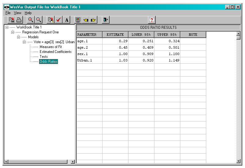
Description of Figure 24 WESVAR fitted model, odds ratios

The output below provides the results of a test of overall fit, along with a test of the contribution of each independent variable to the model, given the other variables are in the model. The test for age is thus testing that the underlying coefficients on the two age dummy variables are simultaneously equal to 0. This is the test that is of interest to the researcher.

Figure 25
WESVAR fitted model output, hypothesis test results

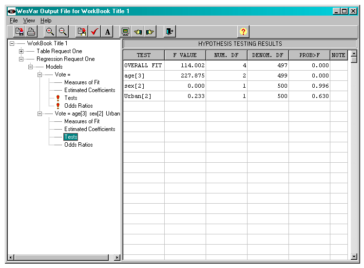
Description of Figure 25 WESVAR fitted model output, hypothesis test results

The output also includes a log that summarizes the logistic regression request. A portion of the log is shown below. This log assists the researcher to check whether the analysis has been carried out as intended.

Figure 26
WESVAR Logistic regression log

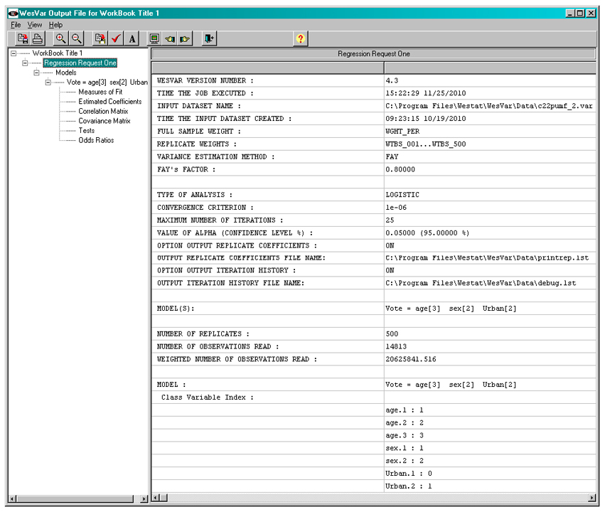
Description of Figure 26 WESVAR Logistic regression log

SAS 9.2

Overview

SAS 9.2 is the first version of SAS that offers some replication approaches to variance estimation in its four survey analysis procedures. The BRR option can be used with user-supplied bootstrap weights in order to obtain bootstrap variance estimates (as explained in Phillips (2004)).

The following table points out the main types of analysis that can be carried out by SAS 9.2, using weighted estimation and bootstrap variance estimation. The names of the particular SAS procedure(s) for obtaining these analyses are also provided.

Table 6
Main types of analysis in SAS 9.2 using survey

As seen from the table and from the SAS 9.2 user guide, several analytic techniques are included within each procedure. It should be noted, however, that variance estimates for percentiles are not available with the BRR option, although the user guide does not point this out. Variance estimates for percentiles, using the BRR option, are available in SAS 9.3.

Software-specific checklist for GSS Example

1. Have you determined the following:

The required weighted estimates and bootstrap variance estimates (errors) are available with the software being used?
SAS can compute the required weighted estimates and bootstrap variance estimates for the types of analysis for the example, and for many other types of analysis as shown in the table above. Choosing the BRR option in SAS for variance estimation and providing the bootstrap weight variables will result in bootstrap variance estimates. The choice of the BRR option with a Fay adjustment can correctly calculate mean bootstrap variance estimates.
Thus, for any SAS procedure the following is required:
1. In the PROC statement, include the varmethod=BRR(FAY=f)option.
  Fay=f is the mean bootstrap adjustment and f should be set to $1 - C^{\frac{1}{2}}$ , where C is the number of bootstrap samples used to produce each mean bootstrap weight variable. (Note: If you have ‘regular’ bootstrap weights rather than mean bootstraps, you just need to include varmethod=BRR in the PROC statement.)
2. Include a WEIGHT statement to identify the weight variable to be used for weighted estimation.
3. Include a REPWEIGHT statement to indicate the names of the bootstrap weight variables on the data file.
  For the particular GSS example, where the weight variable is wght_per, the 500 mean bootstrap weight variables are wtbs_001 to wtbs_500 and each is formed from 25 bootstrap samples, every SAS procedure used would contain the following:
  
  PROC procedurename data=SAS_datafile_name varmethod=BRR(FAY=0.8); WEIGHT wght_per; REPWEIGHT wtbs_001-wtbs_; +Other statements required by the procedure
Have you determined that the required tests/statistics are available with the software being used?
For the GSS example we want to test that each individual model coefficient in the logistic regression is 0, and also that the coefficients on the two age dummy variables are simultaneously 0. The results of such tests are part of the default output from PROC SURVEYLOGISTIC, as demonstrated later. However, it is also possible to request other test statistics to test the same thing or to test more complex relationships among the coefficients of the model.

2. If the specific tests desired are not available, is it possible to write a post-estimation program to calculate them, in the software being used?
It is generally possible to output the SAS results into a SAS data file and then to write a program in SAS to calculate what is required. This was not needed for our example.

3. Is it possible, in the software, to restrict the sample or to remove out-of-sample observations from the full survey data file?
An analysis in SAS can be restricted to the sample with particular characteristics (often called the sample in a particular subpopulation) by the use of a WHERE statement in a SAS procedure. The WHERE statement must be included in every SAS procedure where the restricted sample is required.

Alternatively, it is also straightforward to restrict the sample or remove out-of-sample observations from the full survey data file by writing the code for a DATA step of a SAS program before the call to a SAS survey procedure. This produces a smaller data file that can then be used as the input data file for all SAS procedures where the restricted sample is required.

4. If the survey weight, the bootstrap weights and the analysis variables are not in the same file, do you know how to merge the different sources in the software being used? (This is assuming that the software being used required that all this information be in the same file.)
The merging of the different sources would need to be done in a DATA step or in SQL before the SAS survey procedures are used. SAS, however, does not require that the bootstrap weights be in the same data file as the survey weight and the analysis variables. The SAS user manual gives directions about how to specify a different file for bootstrap weights.

5. While doing your analysis, have you checked the output from the software to determine

that the correct sample size was used
that the correct weight variable was used
that the entire set of bootstrap weights were used
that the mean bootstrap adjustment was correctly implemented (if needed)
whether there are any bootstrap samples for which estimates could not be made?

The default output from a SAS procedure gives the number of observations read and the number of observations used in the analysis carried out by the procedure. It also provides weighted counts of both of those quantities.
The default output from a SAS procedure gives the name of the survey weight variable used.
The default output from a SAS procedure lists number of bootstrap weights that were used.
It can be determined whether the correct mean bootstrap adjustment was made by seeing that the output statement “Fay Coefficient” contains the mean bootstrap adjustment. In the case of GSS 22, this value should be 0.8.
If there are any bootstrap samples for which estimates could not be made, these are identified in the SAS output.

SAS program and output example for GSS

Program

/* PIECE 1 */ options linesize=80; libname pumfl '\\SASD6\Sasd-Dssea-Public\DATA\GSS\DLI\CYCLE22\C22MDFSasAndCode-EngFr';

data c22pumf; set pumfl.c22pumf; run;

/* PIECE 2 */ /*Preliminary descriptive analysis*/ proc surveyfreq data=c22pumf varmethod=BRR(FAY=0.8); tables PER_Q110 ; repweights wtbs_001 - wtbs_500 ; weight wght_per ; run;

/* PIECE 3 */ /*Recode variables and select observations in subpopulation*/ data c22pumf_sub; set pumfl.c22pumf; /*Subpopulation of voters aged 20 to 64*/ if agegr5 ge 03 and agegr5 le 11; if Per_Q110 =1 or Per_Q110 =2; /*Recode of the Urban variable*/ if LUC_RST=1 then Urban=1; else Urban=0; /*Recode of age variable into 3 categories*/ if agegr5 le 04 then age = 1; else if agegr5 le 07 then age =2; else if agegr5 le 11 then age =3; /*Recode of the voted variable*/ if Per_Q110 =1 then Vote =1; else Vote =0; run;

/* PIECE 4 */ proc surveyfreq data=c22pumf_sub varmethod=BRR(FAY=0.8); tables Vote ; repweights wtbs_001 - wtbs_500 ; weight wght_per ; run;

/* PIECE 5 */ /*If rural and sex are included in the class statement without the PARAM=REF option, SAS will use its own coding for the dummy variables (e.g. -1, 1 instead of 0, 1 hence affecting the parameter values)*/ proc surveylogistic data=c22pumf_sub varmethod=BRR(FAY=0.8); class Vote sex(REF=LAST) age(REF=LAST) Urban(REF=LAST) / PARAM=REF; model Vote(event='1')= sex age Urban; repweights wtbs_001 - wtbs_500; weight wght_per; run;

Discussion of Program and Output

PIECE 1

PIECE 2

This piece of the program is a call to PROC SURVEYFREQ for obtaining estimates of the proportions of the full population that made the different types of responses to the question about voting in the last federal election. This allows a preliminary inspection of the variable Per_Q110.

The output provides the method of variance estimation used, the number of replicates used, the sample size and the estimated population size.

As can be seen from the output, 94 % (i.e., 68.98+25.09=94.07) of the population targeted by GSS 22 is estimated to have responded either yes or no to the question on voting in the last federal election. The remainder of the population did not give a yes or no answer for a variety of reasons.

Figure 27
SAS SURVEYFREQ PER_Q110 variable

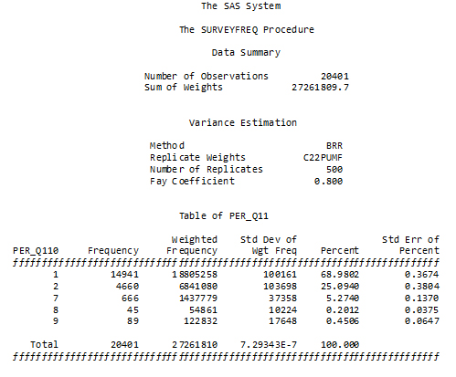
Description of Figure 27 SAS SURVEYFREQ PER_Q110 variable

PIECE 3

Even if it wasn’t the case in the example, it is possible through the TABLES statement of SURVEYFREQ to ask for the coefficient of variation and the confidence limits for a proportion estimate. The limits are by default based on the hypothesis that a ratio of a proportion on it’s standard error folows a t distribution with degrees of freedom equal to the number of bootstrap weights. However, other methods can be chosen to compute a confidence interval as described in the SAS user guide.

PIECE 4

This part of the program is a call to PROC SURVEYFREQ in SAS, to obtain estimates of the percentage of the people aged 20-64 who said “yes” and the percentage who said “no” to the voting question, given that they gave one of these two answers to the question. Note that the new variable VOTE is being used, with the restricted sample. It would have been possible, instead, to have used the full data set but restrict to the subpopulation of interest by including a WHERE statement in PROC SURVEYFREQ.

Figure 28
SAS SURVEYFREQ VOTE variable

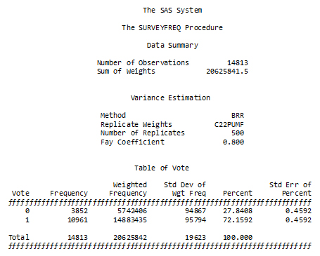
Description of Figure 28 SAS SURVEYFREQ VOTE variable

PIECE 5

This part of the program is the fitting of the logistic model to the restricted sample through a call to PROC SURVEYLOGISTIC in SAS. The procedure is modeling the logit of the probability that VOTE=1 in the restricted sample. Note that all the information about the weight, the bootstrap weights, etc. has to be included in the call to the procedure.

Note that the default output provides information about the categorical variables SEX, AGE, and URBAN, these variables are identified in a CLASS statement

Figure 29
SAS SURVEYLOGISTIC model information

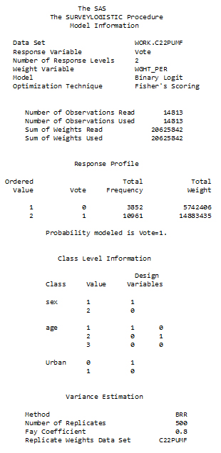
Description of Figure 29 SAS SURVEYLOGISTIC model information

Figure 30
SAS SURVEYLOGISTIC model convergence

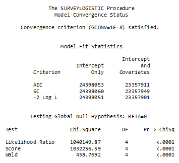
Description of Figure 30 SAS SURVEYLOGISTIC model convergence

The table below provides the result of tests of whether each independent variable contributes significantly to the model. The test statistic for age would be testing whether the underlying coefficients on the two age variables are simultaneously equal to 0, given that the other variables are in the model.

Figure 31
SAS analysis of effects

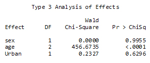
Description of Figure 31 SAS analysis of effects

The fitted model is presented in two forms in two different tables – the first where the fitted coefficients are shown and the other where the coefficients are expressed as odds ratios. Wald chi-square test is used on the model parameters in the first table while confidence intervals are shown for the odds ratio in the second table.

Figure 32
SAS analysis of Maximum Likelihood estimates

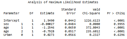
Description of Figure 32 SAS analysis of Maximum Likelihood estimates

Figure 33
SAS odds ratio estimates

Description of Figure 33 SAS odds ratio estimates

BootVar 3.2 for SAS

Overview

The SAS version of BootVar was developed by Statistics Canada methodologists to estimate variances using the bootstrap method. BootVar does not generate bootstrap weights, but uses those provided in the survey data files.

The BootVar macros calculate a variance as the average of the squared differences of the bootstrap estimates from the average of the bootstrap estimates. This is the same as the default method in Stata, while SUDAAN and WesVar calculate a variance as the average of the squared differences of the bootstrap estimates from the full-sample estimate. The two approaches can yield slightly different variance estimates.

The following table points out the main types of analysis that can be carried out by BOOTVAR 3.2, using weighted estimation and bootstrap variance estimation. The name of the particular BOOTVAR macro for obtaining each of these analyses is also provided.

Table 7
Main types of analysis in BootVar 3.2

Details about each macro can be found in the BootVar User Guide, which is accessible when the software is installed. It should be noted that output statistics available from BootVar are more limited than those available from the other software described in this document.

The BootVar User Guide states that “BootVar version 3.2 for SAS has been tested and works with Version 9.1 of SAS. Appropriate results are not guaranteed when using the program with older or more recent versions of SAS.”

Software-specific checklist example for GSS

1. Have you determined the following:

The required weighted estimates and bootstrap variance estimates (errors) are available with the software being used?
BootVar can compute the required weighted estimates and bootstrap variance estimates for the types of analysis for the example, and for many other types of analysis as shown in the table above. The choice of the “R” macro variable can correctly calculate mean bootstrap variance estimates.
For the particular GSS example, the weight variable is wght_per, the 500 mean bootstrap weight variables are wtbs_001 to wtbs_500 and each is formed from 25 standard bootstrap samples. As well, the variable RECID on the data file is a record identifier. Before running any BootVar macro with this data file, the following is required in a SAS program:
1. %let ident = RECID;
  to indicate the name(s) of the unique identification variables for each observation.
2. %let fwgt = wght_per;
  to identify the survey weight variable to be used for weighted estimation.
3. %let bsw = wtbs_;
  to indicate the prefix of the names of the bootstrap weight variables on the data file.
4. %let R = 25;
  to indicate that the bootstrap weight variables are mean bootstrap variables, each created from 25 bootstrap samples. If you have ‘regular’ bootstrap weights, set R to 1.
5. %let B = 500 ;
  the number of bootstrap weights.
The required tests/statistics are available with the software being used?
For the GSS example we want to test that each individual model coefficient in the logistic regression is 0, and also that the coefficients on the two age dummy variables are simultaneously 0. While BootVar provides tests for individual coefficients as part of its default output from %logreg, it does not have the facility to carry out the more complex case of testing whether the coefficients on the 2 age variables are simultaneously 0.

2. If the specific tests desired are not available, is it possible to write a post-estimation program to calculate them, in the software being used?
Quoting from the User Guide: “Since BootVar is distributed as open source code, it is possible for users experienced in SAS programming to modify the program code in order to satisfy needs not addressed by BootVar.”

3. Is it possible, in the software, to restrict the sample or to remove out-of-sample observations from the full survey data file?
An analysis with BootVar can be restricted to the sample with particular characteristics (often called the sample in a particular subpopulation). Restricting the sample or removing out‑of‑sample observations from the full survey data file is done by writing the code for a DATA step of a SAS program before the call to a BootVar macro. This produces a smaller data file that can then be used by BootVar where the restricted sample is required.

4. If the survey weight, the bootstrap weights and the analysis variables are not in the same file, do you know how to merge the different sources in the software being used? (This is assuming that the software being used required that all this information be in the same file.)
BootVar does not require that the survey weight and bootstrap weights be in a different data file than the analysis variables. If they are in different files both files must contain the same unique identifier variables. The researcher does not need to do any merging himself. The names of the analysis file and the file containing the weights must be provided in “%let…” statements before running any BootVar macros. Both %let statements will point to the same file if analysis and weight variables are in the same file.

5. While doing your analysis, have you checked the output from the software to determine:

that the correct sample size was used
that the correct weight variable was used
that the entire set of bootstrap weights were used
that the mean bootstrap adjustment was correctly implemented (if needed)
whether there are any bootstrap samples for which estimates could not be made?

In the SAS log the number of observations used is displayed.
The name of the weight variable used is not displayed
The rep_mod variable tells how many bootstrap weights were used.
The mean bootstrap adjustment is not displayed
If there are any bootstrap samples for which estimates could not be made, this is indicated in the SAS log.

A careful review of the values input in the macro variables is very important with BootVar. There is not much information in the output to verify that the correct parameters were used. One must also check the SAS log to make sure all observations were correctly used.

SAS/BootVar program and output example for GSS

Program

/* PIECE 1 */ libname pumfl ' \\SASD6\Sasd-Dssea-Public\DATA\GSS\DLI\CYCLE22\C22MDFSasAndCode-EngFr'; options linesize=60;

/*From the original data file, produce a new data file that contains the variables required for the first part of the analysis. Some new variables are created. Note that this file also contains the weight variable and the bootstrap weight variables*/

data c22pumf (keep= recid one PER_q110 dp1 dp2 dp7 dp8 dp9 wght_per wtbs_001 - wtbs_500); format per_q110 1. ; set pumfl.c22pumf; one=1; /* Variable with value of 1 for all observations */ /* Create a dummy variable for each different value of PER_Q110 */ if per_q110 =1 then dp1=1; else dp1=0; if per_q110 =2 then dp2=1; else dp2=0; if per_q110 =7 then dp7=1; else dp7=0; if per_q110 =8 then dp8=1; else dp8=0; if per_q110 =9 then dp9=1; else dp9=0; run;

/* PIECE 2 */ /* Estimation of proportions of full population that have the different values of variable Per_Q110, using BootVar */

%let Mfile = c22pumf; %let bsamp = c22pumf; %let classes =.; %let ident = RECID; %let fwgt = wght_per; %let bsw = wtbs_; %let R = 25; %let B = 500 ; %include "F:\DARC\BootVar\MACROE_V32.SAS"; %ratio(dp1,one); %ratio(dp2,one); %ratio(dp7,one); %ratio(dp8,one); %ratio(dp9,one); %output;

/* PIECE 3 */ /* From the original data file, create data file that contains the subpopulation sample for logistic regression. Recode variables needed for the analysis*/

data c22pumf_sub (keep= recid age2034 age3554 sexM Urban Vote one PER_q110 wght_per wtbs_001 - wtbs_500); set pumfl.c22pumf; /*Subpopulation of voters aged 20 to 64*/ if agegr5 ge 03 and agegr5 le 11; if Per_Q110 =1 or Per_Q110 =2; /*Recode the Urban variable*/ if LUC_RST=1 then Urban=1; else Urban=0; /*Recode age variable into 3 categories*/ if agegr5 le 04 then age = 1; else if agegr5 le 07 then age =2; else if agegr5 le 11 then age =3; /*Recode of the voted variable*/ if Per_Q110 =1 then Vote =1; else Vote =0; one=1; /*Create dummy variables for age, needed for logistic regression*/ if age=1 then age2034 = 1; else age2034=0; if age=2 then age3554 = 1; else age3554=0; if sex=1 then sexM=1; else sexM=0; run;

/*PIECE 4*/ /*Estimate proportions with different values of Vote and do logistic regression estimation for variable Vote using BootVar*/ %let Mfile = c22pumf_sub; %let bsamp = c22pumf_sub; %let classes =.; %let ident = RECID; %let fwgt = wght_per; %let bsw = wtbs_; %let R = 25; %let B = 500 ; %include "F:\DARC\BootVar\MACROE_V32.SAS"; %ratio(Vote,one); %logreg(Vote,sexM age2034 age3554 Urban); %output;

Discussion of Program and Output

PIECE 1

This piece of the program is SAS programming, consisting of a data step where a dataset called c22pumf is created from the PUMF SAS dataset. C22pumf has a reduced number of variables in it, which are needed for the estimation of the proportions in the population having the different responses to the voting question. Some of the variables required for the BootVar ratio macro are created in this data step: a variable “one” that takes on the value 1 for all observations, and some 0/1 variables DP1, DP2, etc., one for each possible value of the PER_Q110 variable. In order to create these 0/1 variables, the researcher needs to know the different possible values that PER_Q110 can take on, which he could determine through the data dictionary or through using SAS PROC FREQ. Also retained in C22pumf is RECID, which is a unique record identifier, the survey weight variable wght_per, and all the bootstrap weight variables.

This piece of the program does not produce any output. However, after execution of the data step, the SAS log (not shown) indicates that dataset c22pumf bootstrap_wght contains 20401 records.

PIECE 2

This piece of the program obtains the estimates of the proportions of the full population that made the different types of responses to the question about voting in the last federal election. This allows a preliminary inspection of the variable Per_Q110.

Each estimated proportion requires a separate call to the Bootvar ratio macro. However, if the %output statement is used after the 5 calls to %ratio, the results are displayed in a single table, as seen below.

To estimate the proportion with a specific response, a 0/1 variable needs to be created that takes on the value 1 for records with the specific response in the sample and the value 0 for all other records. This 0/1 variable is then used as the numerator variable in the call to %ratio. For our example, the 0/1 variables for the different responses have the names DP1, DP2, DP7, DP8, and DP9 to correspond to the possible response values of 1,2,7,8,and 9 for Per_Q110.

Since the bootstrap weights are in the same data file as the analysis variables, Mfile and bsamp are set to the same values. If the bootstrap weights had been in a different file than the analysis variables, the values of Mfile and bsamp would have indicated the names of the different files. (For many Statistics Canada surveys, the bootstrap weights are provided in separate files from the analysis variables. However, for GSS22, the PUMF file contains both analysis variables and bootstrap weights.)

Figure 34
SAS BOOTVAR variance estimation for a ratio

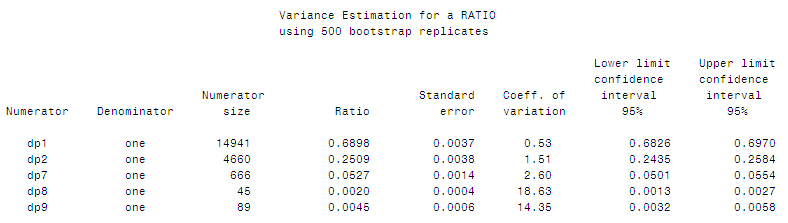
Description of Figure 34 SAS BOOTVAR variance estimation for a ratio

PIECE 3

This piece of the program is a data step in SAS. In it, sample observations in the subpopulation of interest are chosen (i.e., sample observations for people aged 20 to 64 and responding “yes” or “no” to the question about voting). Then, some of the variables are recoded to produce the 0/1 dummy variables that the researcher wishes to use as both dependent and independent variables for the logistic regression since BootVar does not have the facility to do that.

After execution of the data step, the SAS log (not shown) indicates that the new data set c22pumf_sub contains 14813 records. This data step does not produce any output.

PIECE 4

Below is displayed the output from the logistic regression macro. It can be seen in the program that the researcher used the new data set c22pumf_sub as the source for all his analysis variables, for his weights and for his bootstrap weights. The results of the model fitting are displayed in the form of estimated coefficients (in the Beta column of the table) and as odds ratios (in the odds ratio column of the table).

The standard error of each estimated coefficient is provided, along with a Wald statistic for testing whether each coefficient in the model is zero, given that all other variables are in the model. The p value for each Wald test is also displayed. 95% confidence intervals for each odds ratio are also provided.

As noted in the software specific checklist, BootVar does not have the facility for doing a test of whether the two underlying age coefficients in the logistic model are simultaneously zero, after the inclusion of the sex and urban/rural variables in the model.

Figure 35
SAS BOOTVAR variance estimation for a Logistic regression

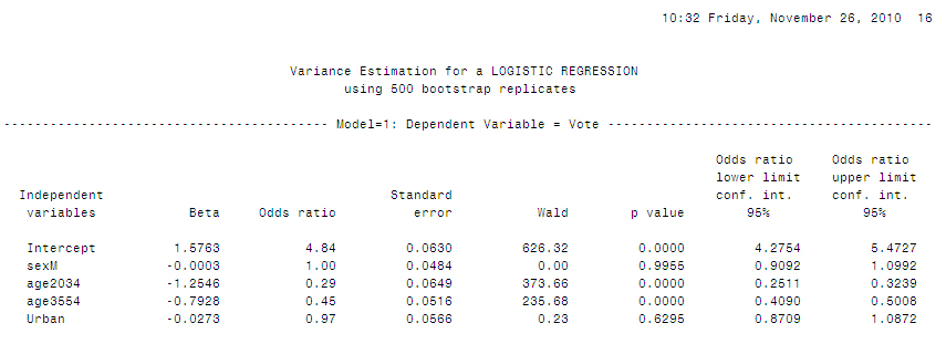
Description of Figure 35 SAS BOOTVAR variance estimation for a Logistic regression

Although not part of the required analysis, another call to the ratio macro was done in this part of the program. This call estimated the proportion of the subpopulation that answered “yes” to the voting question, given that they had answered either “yes” or “no”. In the numerator of the %ratio was the Vote variable that had a value of 1 for people who had answered “yes” and 0 otherwise. The dataset c22pumf_sub contained only records for people who answered “yes” or “no”. The output for this call is given below.

Figure 36
SAS BOOTVAR variance estimation for voting question

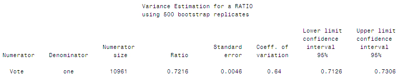
Description of Figure 36 SAS BOOTVAR variance estimation for voting question

References

The list below includes material referred to in this document.

Chowhan, J., and Buckley, N. 2005. Using Mean Bootstrap Weights in Stata: A BSWREG Revision. The Research Data Centres Information and Technical Bulletin, (Spring) Vol. 2 no. 1, 23-37. Statistics Canada Catalogue no. 12-002-XIE.(accessed April 4, 2012).

Phillips, O. 2004. Using Bootstrap Weights with WesVar and SUDAAN. Research Data Centres, Information and Technical Bulletin, Vol. 1 no. 2, 6-15. (accessed July 17, 2013).

The list below includes select books that discuss analysis methods for data from a survey with a complex design.

Chambers, R.L. and Skinner, C.J. (Eds.). 2003. Analysis of Survey Data. John Wiley and Sons.

Cochran, W.G. 1977. Sampling Techniques, 3rd ed., John Wiley and Sons.

Heeringa, S.G., West, B.T., and Berglund, P.A. 2010. Applied Survey Data Analysis. Chapman and Hall / CRC Press.

Korn, E.L. and Graubard, B.I. 1999. Analysis of Health Surveys. John Wiley and Sons.

Lumley, T.S. 2010. Complex Surveys: A Guide to Analysis using R. John Wiley and Sons.

Lohr, S.L. 1999. Sampling: Design and Analysis. Duxbury Press.

Pfeffermann, D. and Rao, C.R. (Eds.). 2010. Handbook of Statistics, Volume 29, Sample Surveys: Inference and Analysis. Elsevier.

Skinner, C.J., Holt, D., and Smith, T.M.F. 1989. Analysis of Complex Surveys. John Wiley and Sons.

Appendix 1 Svy commands in STATA 12, a complete list

The svy prefix can be used with many estimation commands in Stata. Here is the list of estimation commands that support the svy prefix

Descriptive statistics
mean [R] mean — Estimate means
proportion [R] proportion — Estimate proportions
ratio [R] ratio — Estimate ratios
total [R] — Estimate totals
tabulate oneway [svy] tabulate oneway – one way frequency table
tabulate twoway [svy] tabulate twoway – two way frequency table

Linear regression models
cnsreg [R] cnsreg — Constrained linear regression
glm [R] — Generalized linear models
intreg [R] intreg — Interval regression
nl [R] nl — Nonlinear least-squares estimation
regress [R] regress — Linear regression
tobit [R] tobit — Tobit regression
treatreg [R] treatreg — Treatment-effects model
truncreg [R] truncreg — Truncated regression

Survival-data regression models
stcox [ST] stcox — Cox proportional hazards model
streg [ST] streg — Parametric survival models

Binary-response regression models
biprobit [R] biprobit — Bivariate probit regression
cloglog [R] cloglog — Complementary log-log regression
hetprob [R] — Heteroskedastic probit model
logistic [R] logistic — Logistic regression, reporting odds ratios
logit [R] logit — Logistic regression, reporting coefficients
probit [R] probit — Probit regression
scobit [R] scobit — Skewed logistic regression

Discrete-response regression models
clogit [R] clogit — Conditional (fixed-effects) logistic regression
mlogit [R] mlogit — Multinomial (polytomous) logistic regression
mprobit [R] mprobit — Multinomial probit regression
ologit [R] ologit — Ordered logistic regression
oprobit [R] oprobit — Ordered probit regression
slogit [R] slogit — Stereotype logistic regression

Poisson regression models
gnbreg Generalized negative binomial regression in [R] nbreg
nbreg [R] nbreg — Negative binomial regression
poisson [R] poisson — Poisson regression
zinb [R] zinb — Zero-inflated negative binomial regression
zip [R] zip — Zero-inflated Poisson regression
ztnb [R] ztnb — Zero-truncated negative binomial regression
ztp [R] ztp — Zero-truncated Poisson regression

Instrumental-variables regression models
ivprobit [R] ivprobit — Probit model with continuous endogenous regressors
ivregress [R] ivregress — Single-equation instrumental-variables regression
ivtobit [R] ivtobit — Tobit model with continuous endogenous regressors

Regression models with selection
heckman [R] heckman — Heckman selection model
heckprob [R] heckprob — Probit model with sample selection

Appendix 2 STATA before Version 12, how to use weights and bootstrap weights

Version 10

In version 10 of Stata, there needs to be a slight revision to the way that the survey procedures are set up. After this slight revision, all analyses may proceed in an identical manner to that described for Stata 12 in the main part of this manual.

The survey setup command (svyset) needs to be issued with the following specifications:

pweight set to appropriate survey weight variable
Bootstrap weights identified with the brrweight option
Type of variance estimation set to brr with the vce option
Mean square error option set using the mse option. (This option calculates the bootstrap variance as the average of the squared differences between bootstrap estimates and the full-sample estimate. If this option is not selected, the bootstrap variance is computed as the average of the squared differences between the bootstrap estimates and the average of the bootstrap estimates.)
The mean bootstrap adjustment set, if needed, with the Fay option. The value to be entered as the Fay adjustment should be based on a calculation using the following formula:

$1 - C^{\frac{1}{2}}$ , where C is the number of bootstrap samples used to produce each mean bootstrap weight variable.

Version 9

In Version 9, the survey prefix is not available. This drastically changes the procedures to get bootstrapped variance estimates in Stata. These procedures are outline in the RDC Technical Bulletin, Volume 2(1), Spring 2005 in an article entitled Using mean bootstrap weights in Stata: A BSWREG revision by James Chowhan and Neil Buckley.

Appendix 3 SPSS and using bootstrap weights

Although SPSS has an add-on Complex Samples module that offers many survey data analysis tools, one thing that it does not provide is any replication methods for design-based variance estimation. Consequently, SPSS cannot do bootstrap variance estimation using the bootstrap weights provided with many Statistics Canada surveys.

For earlier versions of SPSS, there was an SPSS version of BootVar written by Statistics Canada methodologists that would calculate bootstrap variance estimates for a selection of analytical procedures. This program is no longer being supported or updated.

People who use SPSS for doing other types of analysis thus need to move to a different software package in order to make use of the bootstrap weights. They can choose that package based on their preferred style of doing analysis and on their particular analytical problem. As an example, if a researcher prefers the use of pull-down menus, he could consider WesVar or Stata. Many of the other packages will accept an SPSS datafile as input.

Appendix 4 Normalizing weights

A researcher may have heard about “normalizing” or “scaling” a survey weight variable. By this is meant that the survey weight of each member of the sample in the subpopulation being analysed is divided by the mean of the survey weights for all members of the sample in the subpopulation, i.e., the normalized weight has the value:

$w_{n o r m, i} = \frac{w_{i}}{{\sum_{i \in s_{D}} w_{i}} / n_{D}},$

where w_i is the survey weight for the ith sample member in the subpopulation of interest, S_D represents the sample in this subpopulation, and n_D is the size of this sample. The resulting normalized weights will have an average value of 1.0 and the normalized weights for all sample cases in the subpopulation will add up to n_D, the sample size in the subpopulation.

Normalizing weights is not necessary when analysts use computer software capable of correctly accounting for the survey design in an analysis and when suitable survey design information is available to the analyst. Thus, if an analyst has a survey weight and corresponding bootstrap weights, and if he has appropriate analytical software for survey data, there is no reason for doing any weight normalization.

Why, then, might an analyst not use appropriate software to correctly account for the survey design? Two situations come to mind:

The analyst has survey weights but does not have bootstrap weights or other suitable design information for estimating variances in analytical software for survey data. Thus, analytical software for survey data cannot be used correctly. Such a situation could arise, for example, with a public-use version of a survey data file where, because of confidentiality, only survey weights can be provided.
The analyst has survey weights and corresponding bootstrap weights, but would like to do some preliminary analysis using software other than analytical software for survey data and would also like to use the survey weights. This might occur to save time, or to use some special features of the other software such as some diagnostic graphics capabilities.

Normalizing weights and using these weights in software not specifically for survey data analysis, however, is a stopgap approach. While point estimates can be correct, this approach could lead you to make incorrect conclusions since it is unknown whether the estimated variability measures will be larger or smaller than what would be obtained if a full design-based approach could have been carried out. The size of the estimates of variability affect, for example, the magnitude of test statistics and of p-values and also the width of confidence intervals. While not true in every case, the general tendency is for there to be underestimation of variability measures when a full design-based approach is not taken, which means that p-values tend to be too small and confidence intervals too narrow.

If the analyst has no choice but to use alternative software, he needs to investigate how the alternative software uses a weight variable and whether “better” results would occur if the weight variable were normalized. Two common ways that a non-survey software might treat a weight are

as being a frequency count indicating how many observations have exactly the same values of all variables; or
as being the inverse of the variance of the observation.

Using the weight variable as provided, or after normalizing, will generally give the same point estimates for anything other than the estimate of a total. And these point estimates will be the same as the point estimates that would be obtained from analytical software for survey data. However, where things could be distinctively different between using a normalized and non‑normalized weight in the alternative software would be for estimates of variability and statistical tests based on the variability estimates. Frequently, a normalized weight will produce variability and test results in the alternative software that are closer in value to variability and test results from analytical software for survey data than if a non-normalized weight is used in the alternative software. For this to be the case, though, it is important that the normalizing be done over the sample units in the subpopulation being used in a particular analysis, and not over the full sample of a survey.

In Stata, there are many commands that allow a weight and that are not svy commands. If a pweight can be specified in one of these commands, then normalizing of the weight variable will not have any impact on results.

In SAS, many procedures other than the survey procedures allow a WEIGHT statement. How the weight variable is used in computations varies across those procedures and some of the procedures offer a NORM option. It is advisable to normalize the weight variable in the (sub) sample being used in the analysis by whichever approach is required for the particular procedure being used.

In SPSS, many procedures allow the designation of a weight variable. In most cases, the weights are considered to be frequency weights. Thus, it is advisable to normalize the weight variable in the (sub)sample being used in the analysis.

Date modified:: 2015-11-27