Social Data Linkage Environment (SDLE)

Social Data Linkage Environment (SDLE) information

Overview

Overview of the Social Data Linkage Environment (SDLE)

Derived Record Depository (DRD) linkage status

List of files linked in the Social Data Linkage Environment (SDLE)

Getting started

What to consider before starting a record linkage project at Statistics Canada

Record Linkage Application Process

Record linkage application process: steps to follow

Expanding data potential

The Social Data Linkage Environment (SDLE) at Statistics Canada promotes the innovative use of existing administrative and survey data to address important research questions and inform socio-economic policy through record linkage.

The SDLE expands the potential of data integration across multiple domains, such as health, justice, education and income, through the creation of linked analytical data files without the need to collect additional data from Canadians.

Protecting personal information

Statistics Canada takes your confidentiality very seriously. Under the Statistics Act, all information provided to Statistics Canada is kept confidential, and used only for statistical purposes.

Statistics Canada ensures the privacy and confidentiality and data security of all our programs. In addition to consulting with the Office of the Privacy Commissioner, Statistics Canada conducted a privacy impact assessment to address any potential issues relating to confidentiality or security with the work being undertaken through the SDLE.

Frequently asked questions

What are the benefits of using SDLE?

The SDLE environment offers a highly secure data infrastructure for record linkage activities. It increases efficiency through the use of a processing system, thus offering more timely results and lower costs. SDLE enables linkage across multiple data sets in the social domain which fills important data gaps and can contribute to new research and a better understanding of Canadian society. SDLE also aims to standardize processes, improve methods and enhance data quality.

What services are available?

Our services and supports include: assessing the feasibility of record linkage projects, offering advice on data sources, liaising with subject-matter experts, assisting with approval steps, conducting the record linkage, building custom linked analysis files according to client specifications, advising on analytical limitations and validation, and providing training and outreach.

What kind of linkages can be done in SDLE?

Any linkage of persons can be done in SDLE.

How does SDLE maintain privacy and confidentiality?

Linked analysis files are deemed sensitive statistical information and subject to the confidentiality requirements of the Statistics Act. To reduce the risk of privacy intrusiveness and to minimize the risk of disclosure, source files in SDLE are separated into source index files and source data files. As well, the record linkage production environment that uses the source index files is separated from the data integration and analysis environment that uses the source data files. That is, Statistics Canada employees performing the record linkages in SDLE have access to only the basic personal identifiers needed for linkage. Employees who build the analytical files for research have access only to the data stripped of personal identifiers. Anonymous keys are used to integrate the data from the various sources into a linked analysis data file. Further, only Statistics Canada employees who have an approved need to access the data for their analytical work are allowed access to the linked analysis file. The privacy impact assessment conducted by Statistics Canada found these processes acceptable to reduce the risk of privacy intrusiveness and to minimize the risk of disclosure.

Is there a cost to use SDLE services?

Statistics Canada makes custom services, such as the SDLE, available to Canadian organizations on a cost-recovery basis. Cost-recovery means that clients pay for the direct and indirect cost of doing the work. Custom services are not funded by the budget that Parliament allocates to Statistics Canada. Costs vary depending on the complexity and the requirements of the proposal.

How much does it cost?

The SDLE is a cost-recovery program. Every project is unique and a range of outputs are available. Costs reflect the requirements of each client and range depending on the complexity of the proposal.

How can I get more information on SDLE?

For more information, email us at statcan.sdle-ecds.statcan@statcan.gc.ca.

More information

If you have questions or a potential project for SDLE, please contact us by email at statcan.sdle-ecds.statcan@statcan.gc.ca.

External researchers can access linked analysis files in Statistics Canada's Research Data Centres (RDC). To learn more about the RDC program, please refer to the Research Data Centres program or send an email to statcan.mad-damdam-mad.statcan@statcan.gc.ca.

Permanent Resident Landing File

Description

The Citizenship and Immigration Canada (CIC) permanent resident landing file contains approximately 2.75 million records corresponding to all individuals who landed in Canada during the 2003 – 2013 time frame. The information in the data file is derived from the information included on each individual’s landing record and has not been updated since the time of landing. The variables available may be described using the subjects list below. There are many more variables on the data file because grouped variables have been derived from the landing record data values. For example, age in years is reported on the landing record. An additional two variables corresponding to 5 and 15 year age groups have also been added to the data file. Another example is that the country of birth is reported on the landing record, while an additional two variables which categorize that country into a region of the world and an area of the world have been added to the data file.

Reference period

2003 – 2013

Subjects

  • Age in years, plus 5 year age groups and 15 year age groups
  • Marital Status
  • Gender
  • Mother Tongue
  • Official Languages Spoken
  • Date of Landing: year-month-day
  • Education Level- none, secondary or less, …, doctorate
  • Years Of Schooling
  • Country of Birth, plus grouped categories region & area of the world
  • Country of Citizenship, plus grouped categories region & area of the world
  • intended destination –CMA, census division & province (or if not available, the last known address)
  • Immigration category – provided in first, second, third and fourth level groupings of the immigration category hierarchy
  • Occupation title as listed on the landing record (approximately 9900 categories)
  • Skill levels (two different hierarchies used) corresponding to occupation title as listed on the landing record
  • NOC Code (2006 and 2011) derived from occupation title as listed on the landing record

Target population

A person is included in the database only if he or she obtained landed immigrant or permanent resident status in Canada since 2003 and 2013.

Sampling

Data are collected for all units of the target population, therefore no sampling is done.

Share this page
Date modified:

Description for Chart 1: Comparison of gross budgetary authorities and expenditures as of June 30, 2014, and June 30, 2015, in thousands of dollars

This bar graph shows Statistics Canada's budgetary authorities and expenditures, in thousands of dollars, as of June 30, 2014 and 2015:

  • As at June 30, 2014
    • Net budgetary authorities: $379,555
    • Vote netting authority: $120,000
    • Total authority: $499,555
    • Net expenditures for the period ending June 30: $121,613
    • Year-to-date revenues spent from vote netting authority for the period ending June 30: $12,951
    • Total expenditures: $134,564
  • As at June 30, 2015
    • Net budgetary authorities: $525,095
    • Vote netting authority: $120,000
    • Total authority: $645,095
    • Net expenditures for the period ending June 30: $127,586
    • Year-to-date revenues spent from vote netting authority for the period ending June 30: $5,955
    • Total expenditures: $133,541


Statement outlining results, risks and significant changes in operations, personnel and program

A) Introduction

Statistics Canada's mandate

Statistics Canada is a member of the Industry portfolio.

Statistics Canada's role is to ensure that Canadians have access to a trusted source of statistics on Canada that meets their highest priority needs.

The Agency's mandate derives primarily from the Statistics Act. The Act requires that the Agency collects, compiles, analyzes and publishes statistical information on the economic, social, and general conditions of the country and its people. It also requires that Statistics Canada conduct the census of population and the census of agriculture every fifth year, and protects the confidentiality of the information with which it is entrusted.

Statistics Canada also has a mandate to co-ordinate and lead the national statistical system. The Agency is considered a leader, among statistical agencies around the world, in co-ordinating statistical activities to reduce duplication and reporting burden.

More information on Statistics Canada's mandate, roles, responsibilities and programs can be found in the 2015–2016 Main Estimates and in the Statistics Canada 2015–2016 Report on Plans and Priorities.

The quarterly financial report

  • should be read in conjunction with the 2015–2016 Main Estimates;
  • has been prepared by management, as required by Section 65.1 of the Financial Administration Act, and in the form and manner prescribed by Treasury Board;
  • has not been subject to an external audit or review.

Statistics Canada has the authority to collect and spend revenue from other government departments and agencies, as well as from external clients, for statistical services and products.

Basis of presentation

This quarterly report has been prepared by management using an expenditure basis of accounting. The accompanying Statement of Authorities includes the Agency's spending authorities granted by Parliament and those used by the Agency consistent with the Main Estimates for the 2015–2016 fiscal year. This quarterly report has been prepared using a special purpose financial reporting framework designed to meet financial information needs with respect to the use of spending authorities.

The authority of Parliament is required before moneys can be spent by the Government. Approvals are given in the form of annually approved limits through appropriation acts or through legislation in the form of statutory spending authority for specific purposes.

The Agency uses the full accrual method of accounting to prepare and present its annual departmental financial statements that are part of the departmental performance reporting process. However, the spending authorities voted by Parliament remain on an expenditure basis.

B) Highlights of fiscal quarter and fiscal year-to-date results

This section highlights the significant items that contributed to the net increase in resources available for the year, as well as actual expenditures for the quarter ended June 30.

Description for Chart 1

Comparison of gross budgetary authorities and expenditures as of June 30, 2014, and June 30, 2015, in thousands of dollars

Chart 1 outlines the gross budgetary authorities, which represent the resources available for use for the year as of June 30.

Significant changes to authorities

Total authorities available for 2015–2016 have increased by $145.5 million, or 38%, from the previous year, from $499.6 million to $645.1 million (Chart 1). This net increase was mostly the result of the following:

  • increase for the 2016 Census of Population Program ($141.9 million), as well as for the 2016 Census of Agriculture ($7.2 million)
  • decrease for the 2011 Census of Population Program ($2.8 million), as the program is complete.

In addition to the appropriations allocated to the Agency through the Main Estimates, Statistics Canada also has vote net authority within Vote 105, which entitles the Agency to spend revenues collected from other government departments, agencies, and external clients to provide statistical services. Vote netting authority is stable at $120 million in each of the fiscal years 2014–2015 and 2015–2016.

Significant changes to expenditures

Year-to-date net expenditures recorded to the end of the first quarter increased by $6.0 million, or 4.9%, from $121.6 million to $127.6 million. (See Table A: Variation in Departmental Expenditures by Standard Object.)

Statistics Canada spent approximately 24% of its authorities by the end of the first quarter, compared with 32% in the same quarter of 2014–2015.

Table A: Variation in Departmental Expenditures by Standard Object (unaudited)
This table displays the variance of departmental expenditures by standard object between fiscal year 2014-2015 and 2015-2016. The variance is calculated for year to date expenditures as at the end of the first quarter. The row headers provide information by standard object. The column headers provide information in thousands of dollars and percentage variance for the year to date variation.
Departmental Expenditures Variation by Standard Object Q1 year-to-date variation between fiscal year 2014-2015 and 2015-2016
$'000 %
(01) Personnel 10,244 9.2
(02) Transportation and communications 240 11.6
(03) Information 993 813.9
(04) Professional and special services (243) (8.1)
(05) Rentals (76) (2.2)
(06) Repair and maintenance 10 12.8
(07) Utilities, materials and supplies (45) (12.2)
(08) Acquisition of land, buildings and works - -
(09) Acquisition of machinery and equipment 1,199 637.8
(10) Transfer payments - -
(12) Other subsidies and payments (13,345) (99.6)
Total gross budgetary expenditures (1,023) (0.8)
Less revenues netted against expenditures
Revenues (6,996) (54.0)
Total net budgetary expenditures 5,973 4.9

01) Personnel: The increase was mainly the result of the arbitration award for interviewers and increased collection activities related to cost recovery projects.

03) Information: The increase was the result of the coding review of the standard object definitions and inclusions (e.g., data purchases).

09) Acquisition of machinery and equipment: The increase was the result of timing differences between years for the acquisition of computer equipment.

12) Other subsidies and payments: The decrease is a result of the one-time transition payment for implementing salary payment in arrears made in the first quarter of 2014–2015 by the Government of Canada.

Revenues: The decrease is primarily the result of timing differences between years for the receipt of funds related to the census cost-sharing agreement with another government department.

C) Risks and uncertainties

In 2015–2016, Statistics Canada plans to continue to monitor budget pressures, including the cost saving measures announced in Budget 2014, with the following actions and mitigation strategies:

  • additional analysis, monitoring and validation of financial and human resources information through a monthly financial review by budget holders
  • review of monthly project dashboards in place across the Agency to monitor project issues, risks and alignment with approved budgets
  • continued realignment and reprioritization of work.

In addition, Statistics Canada uses risk management and a risk-based decision-making process to prioritize and conduct its business. In order to effectively do so the Agency identifies its key risks and develops corresponding mitigation strategies in its Corporate Risk Profile.

D) Significant changes to operations, personnel and programs

There have been no significant changes in relation to operations, personnel and programs over the last quarter. For the coming quarters, there will be notable changes in the operations due to increased activities related to the 2016 Census of Population Program.

Approval by senior officials

The original version was signed by
Wayne R. Smith, Chief Statistician
Stéphane Dufour, Chief Financial Officer
Date signed August 27, 2015

Departmental budgetary expenditures by Standard Object (unaudited) - Fiscal year 2015-2016
This table displays the departmental expenditures by standard object for the fiscal year 2015-2016. The row headers provide information by standard object for expenditures and revenues. The column headers provide information in thousands of dollars for planned expenditures for the year ending March 31; expended during the quarter ended June 30; and year to date used at quarter-end 2015-2016.
  Fiscal year 2015-2016
Planned expenditures for the year ending March 31, 2016 Expended during the quarter ended June 30, 2015 Year-to-date used at quarter-end
in tbl-2_housands of dollars
Expenditures
(01) Personnel 480,260 122,145 122,145
(02) tbl-2_ransportation and communications 37,170 2,315 2,315
(03) Information 16,696 1,115 1,115
(04) Professional and special services 54,455 2,758 2,758
(05) Rentals 24,467 3,350 3,350
(06) Repair and maintenance 7,280 88 88
(07) Utilities, materials and supplies 10,685 325 325
(08) Acquisition of land, buildings and works - - -
(09) Acquisition of machinery and equipment 13,901 1,387 1,387
(10) tbl-2_ransfer payments 100 - -
(12) Other subsidies and payments 81 58 58
Total gross budgetary expenditures 645,095 133,541 133,541
Less revenues netted against expenditures
Revenues 120,000 5,955 5,955
Total revenues netted against expenditures 120,000 5,955 5,955
Total net budgetary expenditures 525,095 127,586 127,586
Departmental budgetary expenditures by Standard Object (unaudited) - Fiscal year 2014-2015
This table displays the departmental expenditures by standard object for the fiscal year 2014-2015. The row headers provide information by standard object for expenditures and revenues. The column headers provide information in thousands of dollars for planned expenditures for the year ending March 31; expended during the quarter ended June 30; and year to date used at quarter-end 2014-2015.
  Fiscal year 2014-2015
Planned expenditures for the year ending March 31, 2015 Expended during the quarter ended June 30, 2014 Year-to-date used at quarter-end
in thousands of dollars
Expenditures
(01) Personnel 401,121 111,901 111,901
(02) Transportation and communications 25,808 2,075 2,075
(03) Information 2,509 122 122
(04) Professional and special services 35,680 3,001 3,001
(05) Rentals 13,154 3,426 3,426
(06) Repair and maintenance 7,044 78 78
(07) Utilities, materials and supplies 13,241 370 370
(08) Acquisition of land, buildings and works - - -
(09) Acquisition of machinery and equipment 825 188 188
(10) Transfer payments - - -
(12) Other subsidies and payments 173 13,403 13,403
Total gross budgetary expenditures 499,555 134,564 134,564
Less revenues netted against expenditures
Revenues 120,000 12,951 12,951
Total revenues netted against expenditures 120,000 12,951 12,951
Total net budgetary expenditures 379,555 121,613 121,613
Statement of Authorities (unaudited) - Fiscal year 2015-2016
This table displays the departmental authorities for the fiscal year 2015-2016. The row headers provide information by type of authority, Vote 105 – Net operating expenditures, Statutory authority and Total Budgetary authorities. The column headers provide information in thousands of dollars for Total available for use for the year ending March 31; used during the quarter ended June 30; and year to date used at quarter-end for 2015-2016.
  Fiscal year 2015-2016
Total available for use for the year ending March 31, 2016* Used during the quarter ended June 30, 2015 Year to date used at quarter-end
in thousands of dollars
Vote 105 – Net operating expenditures 456,017 110,316 110,316
Statutory authority – Contribution to employee benefit plans 69,078 17,270 17,270
Total budgetary authorities 525,095 127,586 127,586
Statement of Authorities (unaudited) - Fiscal year 2014-2015
This table displays the departmental authorities for the fiscal year 2014-2015. The row headers provide information by type of authority, Vote 105 – Net operating expenditures, Statutory authority and Total Budgetary authorities. The column headers provide information in thousands of dollars for Total available for use for the year ending March 31; Used during the quarter ended June 30; and year to date used at quarter-end for 2014-2015
  Fiscal year 2014-2015
Total available for use for the year ended March 31, 2015* Used during the quarter ended June 30, 2014 Year to date used at quarter-end
in thousands of dollars
Vote 105 – Net operating expenditures 322,744 107,410 107,410
Statutory authority – Contribution to employee benefit plans 56,811 14,203 14,203
Total budgetary authorities 379,555 121,613 121,613

Trend-cycle estimates – Frequently asked questions

By Susie Fortier, Steve Matthews and Guy Gellatly, Statistics Canada

Statistics Canada releases graphical information on trend-cycle movements for several monthly economic indicators. Estimates of the trend-cycle are presented along with the seasonally adjusted data in selected charts in The Daily. The inclusion of trend-cycle information is intended to support the analysis and interpretation of the seasonally adjusted data.

This reference document provides information on trend-cycle data. It outlines basic concepts and definitions and discusses selected issues related to the use and interpretation of trend-cycle estimates. The document includes a specific example using data on monthly retail sales. Detailed information on the computation of the trend-cycle is also provided.

  1. 1. What is the trend-cycle of a time series?

    Trend-cycle data represent a smoothed version of a seasonally adjusted time series. They provide information on longer-term movements, including changes in direction underlying the series.

    The trend-cycle is the combination of two distinct components:

    • The trend provides information on longer-term movements in the seasonally adjusted data series over several years.
    • The cycle is a sequence of smoother fluctuations around the longer-term trend in part characterized by alternating periods of expansion and contraction.

    Changes in trend-cycle data reflect the influence of factors that condition long-run movements in the economic indicator over time, along with fluctuations in economic activity associated with the business cycle. These two components, the trend and the cycle, are often paired together because of the difficulty involved in estimating them individually.

  2. 2. What is the difference between a seasonally adjusted series and its trend-cycle?

    A seasonally adjusted data series is a series that has been modified to eliminate the effect of seasonal and calendar influences in order to facilitate comparisons of underlying conditions from period to period. Seasonally adjusted data series can also be defined as the combination of the trend-cycle and the irregular component of a time series.

    In much the same way as a seasonally adjusted series represents the raw series with seasonal and calendar effects removed, the trend-cycle estimates represent the seasonally adjusted series with the irregular component removed. As its name suggests, the irregular component is the part of the time series that is not in line with the usual or expected pattern of the series. This irregular component is not part of the trend-cycle, nor is it related to current seasonal factors or calendar effects.

    The irregular component of a time series can represent unanticipated economic events or shocks (for example, strikes, disruptions, natural disasters, unseasonable weather, etc.) or can simply arise from noise in the measurement of the unadjusted data. In some cases, this irregular component can make large contributions to the period-to-period movements in a seasonally adjusted time series.

    By removing this irregular component from seasonally adjusted data, the trend-cycle data can yield a better picture of longer-term movements in the time series. In this sense, the trend-cycle can be interpreted as a smoothed version of the seasonally adjusted series.

  3. 3. What can we learn from trend-cycles?

    Trend-cycle data provide information on longer-term movements in a seasonally adjusted time series, including changes in the direction of the data. These smoothed data make it easier to identify periods of positive change (growth) or negative change (decline) in the time series, as the noise of the irregular component has been removed. This allows for a more accurate identification of turning points in the data.

    For example, the accompanying graph presents data on monthly retail sales in Canada from July 2010 to July 2015. Two data lines are shown: the seasonally adjusted time series and the trend-cycle estimates. The trend-cycle estimates for the most recent reference months are more subject to revision than the estimates for previous periods, and are presented as a dotted line (see question 5).

    While the seasonally adjusted data can be used to examine basic changes in the direction of the time series, it is easier to see the longer term movement in these data from the trend-cycle line. The trend-cycle estimates show that retail sales trended upward at a relatively constant rate during 2010 and 2011, and then slowed in 2012. Growth resumed from late 2012 until mid-2014, before sales trended downward in late 2014. Trend-cycle data for early 2015 indicated a return to growth. Estimates for this most recent period are based on a preliminary estimation of the trend-cycle and should be interpreted with caution as they are subject to revision as noted above.

    Figure 1 — Retail sales

    Trend-cycle - Retail sales

    Sources: CANSIM tables 080-0020 extracted on October 14, 2015; and trend-cycle computations.

    Description for Figure 1
    Table 1 — Retail sales
      $ billion
    Seasonally adjusted Trend-cycle
    July 2010 36.295 36.51
    August 2010 36.515 36.64
    September 2010 36.633 36.79
    October 2010 36.880 36.97
    November 2010 37.568 37.15
    December 2010 37.393 37.30
    January 2011 37.392 37.45
    February 2011 37.438 37.55
    March 2011 37.617 37.64
    April 2011 37.755 37.73
    May 2011 37.724 37.81
    June 2011 38.228 37.92
    July 2011 37.926 38.03
    August 2011 37.977 38.18
    September 2011 38.182 38.34
    October 2011 38.624 38.54
    November 2011 38.780 38.74
    December 2011 39.088 38.89
    January 2012 39.069 38.99
    February 2012 38.942 39.02
    March 2012 39.179 39.00
    April 2012 38.906 38.94
    May 2012 38.774 38.90
    June 2012 38.798 38.89
    July 2012 38.901 38.91
    August 2012 38.918 38.96
    September 2012 39.083 39.04
    October 2012 39.203 39.14
    November 2012 39.314 39.22
    December 2012 39.041 39.31
    January 2013 39.467 39.44
    February 2013 39.673 39.56
    March 2013 39.731 39.72
    April 2013 39.624 39.88
    May 2013 40.337 40.06
    June 2013 40.078 40.25
    July 2013 40.428 40.41
    August 2013 40.612 40.54
    September 2013 40.802 40.67
    October 2013 40.689 40.73
    November 2013 40.929 40.80
    December 2013 40.627 40.88
    January 2014 40.987 41.00
    February 2014 41.196 41.19
    March 2014 41.196 41.41
    April 2014 41.766 41.70
    May 2014 41.840 41.98
    June 2014 42.591 42.27
    July 2014 42.585 42.48
    August 2014 42.419 42.59
    September 2014 42.799 42.61
    October 2014 42.619 42.55
    November 2014 42.886 42.43
    December 2014 42.124 42.28
    January 2015 41.523 42.22
    February 2015 42.184 42.30
    March 2015 42.585 42.45
    April 2015 42.564 42.63*
    May 2015 42.937 42.82*
    June 2015 43.129 43.00*
    July 2015 43.345 43.16*

    Trend-cycle data are particularly useful when the irregular component makes large contributions to the month-to-month movements in a seasonally adjusted time series. In these cases, graphical information on the trend-cycle helps to interpret the movements in the seasonally adjusted series.

  4. 4. Why are trend-cycle data revised?

    Existing estimates of the trend-cycle are revised with each release of new seasonally adjusted data. As new seasonally adjusted data becomes available, the trend-cycle data for previous months can be better estimated. If the trend-cycle data were not revised along with the seasonally adjusted series, the resulting trend-cycle data could contain series breaks, and would likely be inconsistent with the seasonally adjusted series in terms of levels, period-to-period movements, or both. It is necessary to revise the trend-cycle data to maintain their analytical value.

  5. 5. Why is the trend-cycle line dotted for the most recent reference months?

    The trend-cycle line that is published graphically is dotted in the most recent reference periods, as these periods are more likely to be subject to revisions. This is done to signal that the trend-cycle data in this period is a preliminary estimate, and subject to change as new data becomes available. New data make it possible to more accurately estimate the various components that make up the time series. These revisions can change the location of economic turning points, as well as reverse movements between individual months. These types of revisions are more likely to occur in the most recent reference months.

  6. 6. Can the trend-cycle be interpreted as a means of forecasting data for future reference periods?

    The trend-cycle should not be viewed as a way to forecast the underlying seasonally adjusted data. These estimates are based solely on the historical values of the seasonally adjusted series and do not take into account any other information that could be used to project data for future reference periods. Furthermore, since the trend-cycle is subject to revision when additional reference periods are added to the series, the shape of the trend-cycle in the most recent reference periods should be viewed as a preliminary estimate.

  7. 7. What methods can be used to estimate the trend-cycle series?

    There is no unique method that is recommended to estimate the trend-cycle that underlies a time series. A variety of methods have been developed in the literature, ranging from very simple to highly complex. Some methods introduce restrictions on the shape of the trend (for example a linear trend of several years), others are based on explicit models that estimate a trend-cycle component, and others, still, are based on variations of moving averages, where the mean of the data is calculated from successive sub spans or intervals of the data.

    Since the trend-cycle can also be interpreted as a smoothed version of the seasonally adjusted series, a straightforward way of estimating the trend-cycle is by averaging the last three or six months of the data. While this may yield additional insight into the long-term movement in the series, some measure of caution is warranted as this approach does not take the place of more formal trend-cycle estimation techniques. It can be shown that indicators of the economic cycle derived from this simplified method tend to shift in time and may be artificially dampened.

  8. 8. How does Statistics Canada estimate the trend-cycle series?

    Statistics Canada uses a weighted moving average of the data to compute the trend-cycle. This method is based on the Cascade Linear Filter of Dagum and Luati (2008). This weighted average is computed using the previous six months, the current month and (for older estimates) up to six of the subsequent months in the series. In real time, for the most recent reference month in the series, only data for the six previous months and current month are used, as data for subsequent months are not yet known. As these data become available, the trend-cycle estimates will be revised.

    This specific weighted moving average method was selected after an empirical analysis of different alternatives. The estimate of the trend-cycle obtained with the selected method exhibits good statistical properties, as it provides smooth results with limited revisions, and has a low incidence of falsely identifying turning points. As well, it is a linear process and will preserve additive relationship in the data. This implies, for example, that the trend-cycle plotted on employment for men and women separately will sum up to the plotted trend-cycle line for both sexes. The method is easy to replicate as the weights used in the calculation of the weighted average are available.

  9. 9. How does the trend-cycle method work in a more technical sense?

    The trend-cycle is estimated by applying moving averages weighted according to the cascade linear filter to the seasonally adjusted series. In general, the moving average used to calculate the trend-cycle for a specific reference month is a weighted average of up to 13 consecutive months, which are centered on the reference month, where possible.

    For more information on the calculation of trend-cycle estimates, please consult Details on calculation of trend-cycle estimates at Statistics Canada.

  10. 10. How can I learn more about this topic?

    The following references provide more information on the topic of seasonal adjustment, including trend-cycle estimation.

    Dagum, E. B. and Luati, A. 2008. "A Cascade Linear Filter to Reduce Revisions and False Turning Points for Real Time Trend-Cycle Estimation," Econometric Reviews. 28:1-3, 40-59.

    Statistics Canada. 2014. "Seasonally Adjusted Data — Frequently asked questions," Behind the data.

    Statistics Canada. 2009. "Seasonal adjustment and trend-cycle estimation," Statistics Canada Quality Guidelines. 5th edition. Catalogue no. 12-539-X.

Access to microdata

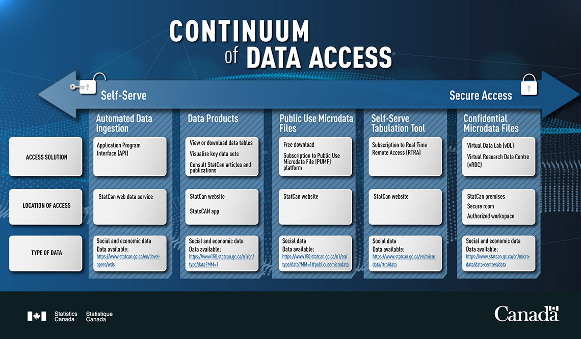
Statistics Canada recognizes that data users require access to microdata at the business, household, or personal level for research purposes. To encourage the use of microdata, Statistics Canada offers a wide range of access solutions through a series of online channels, facilities, and programs for data user's, while at the same time protecting the privacy and confidentiality of respondents. These access solutions are displayed in the continuum of access below, which provides an overview of all types of data available in Statistics Canada. All access solutions prioritize the confidentiality of respondents to ensure that no personal or identifiable information is published.

Continuum of data access

Self-serve access solutions, available with minimal restrictions, progress into secure access solutions, available with security procedures.

Automated data ingestion

A self-serve way to programmatically take away data and reuse it for applications, databases, and analyses.

Access solution

  • Application program interface (API): Allows data users to access Statistics Canada aggregate data and metadata by connecting directly to our public facing databases. The Statistics Canada web services provide access to the time series made available on Statistics Canada's website in a structured form.

Location of access

Type of data

Ideal activities

  • Training
  • Policy research
  • Academic research
  • Evidence-based policy/decision-making
  • Outcomes or products – data exploration, extractions and as an analytical tool for academic and policy research
Data products

Publications, data visualizations, and downloadable items such as multi-dimensional data tables storing standard socio-economic data sets.

Access solution

  • View or download data tables: Data
  • Visualize key data sets: Data
  • Consult StatCan articles and publications: Analysis

Location of access

Type of data

  • Social and economic data: Data

Ideal activities

  • Training
  • Policy research
  • Academic research
  • Evidence-based policy/decision-making – calculating frequencies, cross tabulations, means, percentiles, percent distribution, proportions, ratios, and shares
  • Outcomes or products – data exploration, extractions and as an analytical tool for academic and policy research
Public use microdata files

Access solution

Location of access

Type of data

Ideal activities

  • Training – use as an analytical training tool.
  • Policy research
  • Academic research
  • Evidence-based policy/decision-making – calculating frequencies, cross tabulations, means, percentiles, percent distribution, proportions, ratios, and shares
  • Outcomes or products – data exploration, extractions, and as an analytical tool for academic and policy research
Self-serve tabulation tool

Access solution

Subscription to Real Time Remote Access (RTRA): Indirect access to Statistics Canada's microdata files, to produce non-confidential tabulations, via remotely submitted SAS programs. It is suitable for clients primarily looking for descriptive statistics.

Location of access

Type of data

Ideal activities

  • Training
  • Policy research
  • Academic research
  • Evidence-based policy/decision-making – calculating frequencies, means, percentiles, proportions, ratios, and shares
  • Outcomes or products – generating a full range of descriptive statistics that can be used for academic and policy research, training, and policy briefings
Confidential microdata files

Data at the individual or institutional level accessed in a secured environment.

Access solution

  • Virtual Data Lab (vDL): A secure cloud infrastructure used to store and facilitate access to microdata research projects. The vDL grants qualifying data users a more flexible approach to accessing Statistics Canada microdata. Data users can access their microdata projects from various locations, such as their home or office, depending on the sensitivity of the data.
  • Virtual Research Data Centre (vRDC): A modern virtual infrastructure that will provide academic data users with secure access to Statistics Canada microdata through a partnership with the Canadian Research Data Centre Network (CRDCN). Qualifying data users will have access to data within secure RDC facilities, as well as from other authorized workspaces (e.g., a home or office). The vRDC is expected to start coming online in 2023.

Location of access

  • Secure Access Points: Statistics Canada premises (e.g., Research Data Centres), secure rooms, authorized workspaces (e.g., personal residence)

Type of data

Ideal activities

  • Training
  • Policy research – answering policy and academic research questions that require the use of advanced analytical methods such as complex multivariate analysis, and modelling
  • Academic research
  • Evidence-based policy/decision-making
  • Outcomes or products

Data Access Division newsletter

The Data Access Division newsletter is released on a quarterly basis to inform the user community about various ongoing Divisional initiatives. The newsletter issues are available here:

2023
2022
2021
2020

Self-serve access to microdata

Statistics Canada offers Public Use Microdata Files (PUMFs) to institutions and individuals. They are non-aggregated data which are carefully modified and then reviewed to ensure that no individual or business is directly or indirectly identified. These can be accessed directly through the Data Liberation Initiative (DLI) or the PUMF Collection for a subscription fee. Individual PUMF files can also be downloaded from the website at no cost. Statistics Canada offers remote access solutions to researchers and users.

Public Use Microdata Files Collection

The Public Use Microdata File (PUMF) Collection is a subscription-based service for institutions that require unlimited access to all anonymized and non-aggregated data, which is available through Statistics Canada's Electronic File Transfer Service (EFT) and an Internet Protocol (IP) restricted online database, Rich Data Services, with an easy-to-use discoverability tool. Select files are also available free of charge from the Statistics Canada website.

The Data Liberation Initiative

The Data Liberation Initiative (DLI) is a partnership between postsecondary institutions and Statistics Canada to improve access to Canadian data resources, allowing faculty and students unlimited access to numerous public use data and geographical files.

Real Time Remote Access

Real Time Remote Access (RTRA) is an online tabulation tool allowing subscribers to run SAS programs in real time to extract results from masterfile subsets in the form of tables.

Secure access to microdata

Research Data Centres are secure physical environments available to accredited data users and government employees to access deidentified and non-aggregated microdata for research purposes. Data users have direct access to a wide range of deidentified survey, administrative, and integrated data.

Accredited data users are approved researchers who come from an accredited organization that has indicated in writing to Statistics Canada that the researcher is trustworthy and will follow the security protocols for data access in a Statistics Canada premise and an authorized workspace.

Research Data Centres

Data access for academic data users

Research Data Centres (RDCs) are located on university campuses across Canada and are staffed by Statistics Canada employees. These centres are accessible to accredited data users affiliated with the hosting organization.

Launching in 2024, the virtual Research Data Centre (vRDC) will provide a modern virtual infrastructure that will provide academic researchers with secure access to Statistics Canada microdata through a partnership with the Canadian Research Data Centre Network (CRDCN). Qualifying data users will have access to data within secure RDC facilities, as well as from other "authorized workspaces" (e.g., a home or office location).

All data output is vetted for confidentiality, by Statistics Canada employees, prior to being released to data users.

Data access for government data users

The Federal Research Data Centre (FRDC) provides federal, provincial and municipal government employees and data users from non-government organizations (NGOs) and the private sector with a secure environment to access confidential microdata. The physical FRDC is located in the National Capital Region.

Accredited FRDC users with approved eligible microdata research projects can access confidential microdata remotely, in authorized workspaces, via the virtual Data Lab (vDL). Fees for access vary depending on the project.

All data output is vetted for confidentiality, by Statistics Canada employees, prior to being released to data users.

Statistics Canada Biobank

Biospecimens like blood, urine, and DNA samples are collected from consenting participants of the Canadian Health Measures Survey (CHMS) and are only accessible for approved research initiatives that meet ethical standards. The resulting analyses are made available through the Research Data Centres. Under no circumstances will personal or identifiable information be published. Datasets of potential interest are available to approved academics and government data users.

Approved data users are deemed employees of Statistics Canada who have signed a Microdata Research Contract or a Microdata Service Contract noting their approval to access data for a specified purpose on a Statistics Canada premise.

Concepts, definitions and data quality

The Monthly Survey of Manufacturing (MSM) publishes statistical series for manufacturers – sales of goods manufactured, inventories, unfilled orders and new orders. The values of these characteristics represent current monthly estimates of the more complete Annual Survey of Manufactures and Logging (ASML) data.

The MSM is a sample survey of approximately 10,500 Canadian manufacturing establishments, which are categorized into over 220 industries. Industries are classified according to the 2012 North American Industrial Classification System (NAICS). Seasonally adjusted series are available for the main aggregates.

An establishment comprises the smallest manufacturing unit capable of reporting the variables of interest. Data collected by the MSM provides a current ‘snapshot’ of sales of goods manufactured values by the Canadian manufacturing sector, enabling analysis of the state of the Canadian economy, as well as the health of specific industries in the short- to medium-term. The information is used by both private and public sectors including Statistics Canada, federal and provincial governments, business and trade entities, international and domestic non-governmental organizations, consultants, the business press and private citizens. The data are used for analyzing market share, trends, corporate benchmarking, policy analysis, program development, tax policy and trade policy.

1. Sales of goods manufactured

Sales of goods manufactured (formerly shipments of goods manufactured) are defined as the value of goods manufactured by establishments that have been shipped to a customer. Sales of goods manufactured exclude any wholesaling activity, and any revenues from the rental of equipment or the sale of electricity. Note that in practice, some respondents report financial transactions rather than payments for work done. Sales of goods manufactured are available by 3-digit NAICS, for Canada and broken down by province.

For the aerospace product and parts, and shipbuilding industries, the value of production is used instead of sales of goods manufactured. This value is calculated by adjusting monthly sales of goods manufactured by the monthly change in inventories of goods / work in process and finished goods manufactured. Inventories of raw materials and components are not included in the calculation since production tries to measure "work done" during the month. This is done in order to reduce distortions caused by the sales of goods manufactured of high value items as completed sales.

2. Inventories

Measurement of component values of inventory is important for economic studies as well as for derivation of production values. Respondents are asked to report their book values (at cost) of raw materials and components, any goods / work in process, and finished goods manufactured inventories separately. In some cases, respondents estimate a total inventory figure, which is allocated on the basis of proportions reported on the ASML. Inventory levels are calculated on a Canada‑wide basis, not by province.

3. Orders

a) Unfilled Orders

Unfilled orders represent a backlog or stock of orders that will generate future sales of goods manufactured assuming that they are not cancelled. As with inventories, unfilled orders and new orders levels are calculated on a Canada‑wide basis, not by province.

The MSM produces estimates for unfilled orders for all industries except for those industries where orders are customarily filled from stocks on hand and order books are not generally maintained. In the case of the aircraft companies, options to purchase are not treated as orders until they are entered into the accounting system.

b) New Orders

New orders represent current demand for manufactured products. Estimates of new orders are derived from sales of goods manufactured and unfilled orders data. All sales of goods manufactured within a month result from either an order received during the month or at some earlier time. New orders can be calculated as the sum of sales of goods manufactured adjusted for the monthly change in unfilled orders.

4. Non-Durable / Durable goods

a) Non-durable goods industries include:

Food (NAICS 311),
Beverage and Tobacco Products (312),
Textile Mills (313),
Textile Product Mills (314),
Clothing (315),
Leather and Allied Products (316),
Paper (322),
Printing and Related Support Activities (323),
Petroleum and Coal Products (324),
Chemicals (325) and
Plastic and Rubber Products (326).

b) Durable goods industries include:

Wood Products (NAICS 321),
Non-Metallic Mineral Products (327),
Primary Metals (331),
Fabricated Metal Products (332),
Machinery (333),
Computer and Electronic Products (334),
Electrical Equipment, Appliance and Components (335),
Transportation Equipment (336),
Furniture and Related Products (337) and
Miscellaneous Manufacturing (339).

Survey design and methodology

Concept Review

In 2007, the MSM terminology was updated to be Charter of Accounts (COA) compliant. With the August 2007 reference month release the MSM has harmonized its concepts to the ASML. The variable formerly called “Shipments” is now called “Sales of goods manufactured”. As well, minor modifications were made to the inventory component names. The definitions have not been modified nor has the information collected from the survey.

Methodology

The latest sample design incorporates the 2012 North American Industrial Classification Standard (NAICS). Stratification is done by province with equal quality requirements for each province. Large size units are selected with certainty and small units are selected with a probability based on the desired quality of the estimate within a cell.

The estimation system generates estimates using the NAICS. The estimates will also continue to be reconciled to the ASML. Provincial estimates for all variables will be produced. A measure of quality (CV) will also be produced.

Components of the Survey Design

Target Population and Sampling Frame

Statistics Canada’s business register provides the sampling frame for the MSM. The target population for the MSM consists of all statistical establishments on the business register that are classified to the manufacturing sector (by NAICS). The sampling frame for the MSM is determined from the target population after subtracting establishments that represent the bottom 5% of the total manufacturing sales of goods manufactured estimate for each province. These establishments were excluded from the frame so that the sample size could be reduced without significantly affecting quality.

The Sample

The MSM sample is a probability sample comprised of approximately 10,500 establishments. A new sample was chosen in the autumn of 2012, followed by a six-month parallel run (from reference month September 2012 to reference month February 2013). The refreshed sample officially became the new sample of the MSM effective in December 2012.

This marks the first process of refreshing the MSM sample since 2007. The objective of the process is to keep the sample frame as fresh and up-to date as possible. All establishments in the sample are refreshed to take into account changes in their value of sales of goods manufactured, the removal of dead units from the sample and some small units are rotated out of the GST-based portion of the sample, while others are rotated into the sample.

Prior to selection, the sampling frame is subdivided into industry-province cells. For the most part, NAICS codes were used. Depending upon the number of establishments within each cell, further subdivisions were made to group similar sized establishments’ together (called stratum). An establishment’s size was based on its most recently available annual sales of goods manufactured or sales value.

Each industry by province cell has a ‘take-all’ stratum composed of establishments sampled each month with certainty. This ‘take-all’ stratum is composed of establishments that are the largest statistical enterprises, and have the largest impact on estimates within a particular industry by province cell. These large statistical enterprises comprise 45% of the national manufacturing sales of goods manufactured estimates.

Each industry by province cell can have at most three ‘take-some’ strata. Not all establishments within these stratums need to be sampled with certainty. A random sample is drawn from the remaining strata. The responses from these sampled establishments are weighted according to the inverse of their probability of selection. In cells with take-some portion, a minimum sample of 10 was imposed to increase stability.

The take-none portion of the sample is now estimated from administrative data and as a result, 100% of the sample universe is covered. Estimation of the take-none portion also improved efficiency as a larger take-none portion was delineated and the sample could be used more efficiently on the smaller sampled portion of the frame.

Data Collection

Only a subset of the sample establishments is sent out for data collection. For the remaining units, information from administrative data files is used as a source for deriving sales of goods manufactured data. For those establishments that are surveyed, data collection, data capture, preliminary edit and follow-up of non-respondents are all performed in Statistics Canada regional offices. Sampled establishments are contacted by mail or telephone according to the preference of the respondent. Data capture and preliminary editing are performed simultaneously to ensure the validity of the data.

In some cases, combined reports are received from enterprises or companies with more than one establishment in the sample where respondents prefer not to provide individual establishment reports. Businesses, which do not report or whose reports contain errors, are followed up immediately.

Use of Administrative Data

Managing response burden is an ongoing challenge for Statistics Canada. In an attempt to alleviate response burden, especially for small businesses, Statistics Canada has been investigating various alternatives to survey taking. Administrative data files are a rich source of information for business data and Statistics Canada is working at mining this rich data source to its full potential. As such, effective the August 2004 reference month, the MSM reduced the number of simple establishments in the sample that are surveyed directly and instead, derives sales of goods manufactured data for these establishments from Goods and Services Tax (GST) files using a statistical model. The model accounts for the difference between sales of goods manufactured (reported to MSM) and sales (reported for GST purposes) as well as the time lag between the reference period of the survey and the reference period of the GST file.

Effective from the January 2013 reference month, the MSM derives sales of goods manufactured data for non-incorporated establishments (e.g. the self employed) from T1 files. A statistical model is used to transform T1 data into sales of goods manufactured data.

In conjunction with the most recent sample, effective December 2012, approximately 2,800 simple establishments were selected to represent the GST portion of the sample.

Inventories and unfilled orders estimates for establishments where sales of goods manufactured are GST-based are derived using the MSM’s imputation system. The imputation system applies to the previous month values, the month-to-month and year-to-year changes in similar firms which are surveyed. With the most recent sample, the eligibility rules for GST-based establishments were refined to have more GST-based establishments in industries that typically carry fewer inventories. This way the impact of the GST-based establishments which require the estimation of inventories, will be kept to a minimum.

Detailed information on the methodology used for modelling sales of goods manufactured from administrative data sources can be found in the ‘Monthly Survey of Manufacturing: Use of Administrative Data’ (Catalogue no. 31-533-XIE) document.

Data quality

Statistical Edit and Imputation

Data are analyzed within each industry-province cell. Extreme values are listed for inspection by the magnitude of the deviation from average behavior. Respondents are contacted to verify extreme values. Records that fail statistical edits are considered outliers and are not used for imputation.

Values are imputed for the non-responses, for establishments that do not report or only partially complete the survey form. A number of imputation methods are used depending on the variable requiring treatment. Methods include using industry-province cell trends, historical responses, or reference to the ASML. Following imputation, the MSM staff performs a final verification of the responses that have been imputed.

Revisions

In conjunction with preliminary estimates for the current month, estimates for the previous three months are revised to account for any late returns. Data are revised when late responses are received or if an incorrect response was recorded earlier.

Estimation

Estimates are produced based on returns from a sample of manufacturing establishments in combination with administrative data for a portion of the smallest establishments. The survey sample includes 100% coverage of the large manufacturing establishments in each industry by province, plus partial coverage of the medium and small-sized firms. Combined reports from multi-unit companies are pro-rated among their establishments and adjustments for progress billings reflect revenues received for work done on large item contracts. Approximately 2,800 of the sampled medium and small-sized establishments are not sent questionnaires, but instead their sales of goods manufactured are derived by using revenue from the GST files. The portion not represented through sampling – the take-none portion - consist of establishments below specified thresholds in each province and industry. Sub-totals for this portion are also derived based on their revenues.

Industry values of sales of goods manufactured, inventories and unfilled orders are estimated by first weighting the survey responses, the values derived from the GST files and the imputations by the number of establishments each represents. The weighted estimates are then summed with the take-none portion. While sales of goods manufactured estimates are produced by province, no geographical detail is compiled for inventories and orders since many firms cannot report book values of these items monthly.

Benchmarking

Up to and including 2003, the MSM was benchmarked to the Annual Survey of Manufactures and Logging (ASML). Benchmarking was the regular review of the MSM estimates in the context of the annual data provided by the ASML. Benchmarking re-aligned the annualized level of the MSM based on the latest verified annual data provided by the ASML.

Significant research by Statistics Canada in 2006-2007 was completed on whether the benchmark process should be maintained. The conclusion was that benchmarking of the MSM estimates to the ASML should be discontinued. With the refreshing of the MSM sample in 2007, it was determined that benchmarking would no longer be required (retroactive to 2004) because the MSM now accurately represented 100% of the sample universe. Data confrontation will continue between MSM and ASML to resolve potential discrepancies.

As of the December 2012 reference month, a new sample was introduced. It is standard practice that every few years the sample is refreshed to ensure that the survey frame is up to date with births, deaths and other changes in the population. The refreshed sample is linked at the detailed level to prevent data breaks and to ensure the continuity of time series. It is designed to be more representative of the manufacturing industry at both the national and provincial levels.

Data confrontation and reconciliation

Each year, during the period when the Annual Survey of Manufactures and Logging section set their annual estimates, the MSM section works with the ASML section to confront and reconcile significant differences in values between the fiscal ASML and the annual MSM at the strata and industry level.

The purpose of this exercise of data reconciliation is to highlight and resolve significant differences between the two surveys and to assist in minimizing the differences in the micro-data between the MSM and the ASML.

Sampling and Non-sampling Errors

The statistics in this publication are estimates derived from a sample survey and, as such, can be subject to errors. The following material is provided to assist the reader in the interpretation of the estimates published.

Estimates derived from a sample survey are subject to a number of different kinds of errors. These errors can be broken down into two major types: sampling and non-sampling.

1. Sampling Errors

Sampling errors are an inherent risk of sample surveys. They result from the difference between the value of a variable if it is randomly sampled and its value if a census is taken (or the average of all possible random values). These errors are present because observations are made only on a sample and not on the entire population.

The sampling error depends on factors such as the size of the sample, variability in the population, sampling design and method of estimation. For example, for a given sample size, the sampling error will depend on the stratification procedure employed, allocation of the sample, choice of the sampling units and method of selection. (Further, even for the same sampling design, we can make different calculations to arrive at the most efficient estimation procedure.) The most important feature of probability sampling is that the sampling error can be measured from the sample itself.

2. Non-sampling Errors

Non-sampling errors result from a systematic flaw in the structure of the data-collection procedure or design of any or all variables examined. They create a difference between the value of a variable obtained by sampling or census methods and the variable’s true value. These errors are present whether a sample or a complete census of the population is taken. Non-sampling errors can be attributed to one or more of the following sources:

a) Coverage error: This error can result from incomplete listing and inadequate coverage of the population of interest.

b) Data response error: This error may be due to questionnaire design, the characteristics of a question, inability or unwillingness of the respondent to provide correct information, misinterpretation of the questions or definitional problems.

c) Non-response error: Some respondents may refuse to answer questions, some may be unable to respond, and others may be too late in responding. Data for the non-responding units can be imputed using the data from responding units or some earlier data on the non-responding units if available.

The extent of error due to imputation is usually unknown and is very much dependent on any characteristic differences between the respondent group and the non-respondent group in the survey. This error generally decreases with increases in the response rate and attempts are therefore made to obtain as high a response rate as possible.

d) Processing error: These errors may occur at various stages of processing such as coding, data entry, verification, editing, weighting, and tabulation, etc. Non-sampling errors are difficult to measure. More important, non-sampling errors require control at the level at which their presence does not impair the use and interpretation of the results.

Measures have been undertaken to minimize the non-sampling errors. For example, units have been defined in a most precise manner and the most up-to-date listings have been used. Questionnaires have been carefully designed to minimize different interpretations. As well, detailed acceptance testing has been carried out for the different stages of editing and processing and every possible effort has been made to reduce the non-response rate as well as the response burden.

Measures of Sampling and Non-sampling Errors

1. Sampling Error Measures

The sample used in this survey is one of a large number of all possible samples of the same size that could have been selected using the same sample design under the same general conditions. If it was possible that each one of these samples could be surveyed under essentially the same conditions, with an estimate calculated from each sample, it would be expected that the sample estimates would differ from each other.

The average estimate derived from all these possible sample estimates is termed the expected value. The expected value can also be expressed as the value that would be obtained if a census enumeration were taken under identical conditions of collection and processing. An estimate calculated from a sample survey is said to be precise if it is near the expected value.

Sample estimates may differ from this expected value of the estimates. However, since the estimate is based on a probability sample, the variability of the sample estimate with respect to its expected value can be measured. The variance of an estimate is a measure of the precision of the sample estimate and is defined as the average, over all possible samples, of the squared difference of the estimate from its expected value.

The standard error is a measure of precision in absolute terms. The coefficient of variation (CV), defined as the standard error divided by the sample estimate, is a measure of precision in relative terms. For comparison purposes, one may more readily compare the sampling error of one estimate to the sampling error of another estimate by using the coefficient of variation.

In this publication, the coefficient of variation is used to measure the sampling error of the estimates. However, since the coefficient of variation published for this survey is calculated from the responses of individual units, it also measures some non-sampling error.

The formula used to calculate the published coefficients of variation (CV) in Table 1 is:

CV(X) = S(X)/X

where X denotes the estimate and S(X) denotes the standard error of X.

In this publication, the coefficient of variation is expressed as a percentage.

Confidence intervals can be constructed around the estimate using the estimate and the coefficient of variation. Thus, for our sample, it is possible to state with a given level of confidence that the expected value will fall within the confidence interval constructed around the estimate. For example, if an estimate of $12,000,000 has a coefficient of variation of 10%, the standard error will be $1,200,000 or the estimate multiplied by the coefficient of variation. It can then be stated with 68% confidence that the expected value will fall within the interval whose length equals the standard deviation about the estimate, i.e., between $10,800,000 and $13,200,000. Alternatively, it can be stated with 95% confidence that the expected value will fall within the interval whose length equals two standard deviations about the estimate, i.e., between $9,600,000 and $14,400,000.

Text table 1 contains the national level CVs, expressed as a percentage, for all manufacturing for the MSM characteristics. For CVs at other aggregate levels, contact the Dissemination and Frame Services Section at (613) 951-9497, toll free: 1-866-873-8789 or by e-mail at manufact@statcan.gc.ca.

Text table 1
National Level CVs by Characteristic
Table summary
This table displays the results of National Level CVs by Characteristic. The information is grouped by MONTH (appearing as row headers), Sales of goods manufactured, Raw materials and components inventories, Goods / work in process inventories, Finished goods manufactured inventories and Unfilled Orders, calculated using % units of measure (appearing as column headers).
MONTH Sales of goods manufactured Raw materials and components inventories Goods / work in process inventories Finished goods manufactured inventories Unfilled Orders
%
March 2015 0.55 1.06 0.93 1.07 0.65
April 2015 0.53 1.02 0.93 1.08 0.67
May 2015 0.51 1.02 0.96 1.10 0.60
June 2015 0.50 1.00 0.98 1.13 0.62
July 2015 0.53 1.04 0.95 1.13 0.59
August 2015 0.54 1.00 0.94 1.15 0.64
September 2015 0.55 1.03 0.96 1.17 0.66
October 2015 0.56 1.01 0.93 1.15 0.64
November 2015 0.54 1.01 0.89 1.12 0.62
December 2015 0.57 1.02 0.92 1.14 0.65
January 2016 0.57 1.07 0.86 1.16 0.65
February 2016 0.60 1.08 0.88 1.17 0.65
March 2016 0.62 1.15 0.93 1.17 0.64

2. Non-sampling Error Measures

The exact population value is aimed at or desired by both a sample survey as well as a census. We say the estimate is accurate if it is near this value. Although this value is desired, we cannot assume that the exact value of every unit in the population or sample can be obtained and processed without error. Any difference between the expected value and the exact population value is termed the bias. Systematic biases in the data cannot be measured by the probability measures of sampling error as previously described. The accuracy of a survey estimate is determined by the joint effect of sampling and non-sampling errors.

Sources of non-sampling error in the MSM include non-response error, imputation error and the error due to editing. To assist users in evaluating these errors, weighted rates are given in Text table 2. The following is an example of what is meant by a weighted rate. A cell with a sample of 20 units in which five respond for a particular month would have a response rate of 25%. If these five reporting units represented $8 million out of a total estimate of $10 million, the weighted response rate would be 80%.

The definitions for the weighted rates noted in Text table 2 follow. The weighted response and edited rate is the proportion of a characteristic’s total estimate that is based upon reported data and includes data that has been edited. The weighted imputation rate is the proportion of a characteristic’s total estimate that is based upon imputed data. The weighted GST data rate is the proportion of the characteristic’s total estimate that is derived from Goods and Services Tax files (GST files). The weighted take-none fraction rate is the proportion of the characteristic’s total estimate modeled from administrative data.

Text table 2 contains the weighted rates for each of the characteristics at the national level for all of manufacturing. In the table, the rates are expressed as percentages.

Text Table 2
National Weighted Rates by Source and Characteristic
Table summary
This table displays the results of National Weighted Rates by Source and Characteristic. The information is grouped by Characteristics (appearing as row headers), Data source, Response or edited, Imputed, GST data and Take-none fraction, calculated using % units of measure (appearing as column headers).
Characteristics Data source
Response or edited Imputed GST data Take-none fraction
%
Sales of goods manufactured 83.9 4.5 7.2 4.4
Raw materials and components 76.9 17.8 0.0 5.3
Goods / work in process 82.4 13.5 0.0 4.0
Finished goods manufactured 78.1 16.9 0.0 5.1
Unfilled Orders 92.3 4.4 0.0 3.3

Joint Interpretation of Measures of Error

The measure of non-response error as well as the coefficient of variation must be considered jointly to have an overview of the quality of the estimates. The lower the coefficient of variation and the higher the weighted response rate, the better will be the published estimate.

Seasonal Adjustment

Economic time series contain the elements essential to the description, explanation and forecasting of the behavior of an economic phenomenon. They are statistical records of the evolution of economic processes through time. In using time series to observe economic activity, economists and statisticians have identified four characteristic behavioral components: the long-term movement or trend, the cycle, the seasonal variations and the irregular fluctuations. These movements are caused by various economic, climatic or institutional factors. The seasonal variations occur periodically on a more or less regular basis over the course of a year. These variations occur as a result of seasonal changes in weather, statutory holidays and other events that occur at fairly regular intervals and thus have a significant impact on the rate of economic activity.

In the interest of accurately interpreting the fundamental evolution of an economic phenomenon and producing forecasts of superior quality, Statistics Canada uses the X12-ARIMA seasonal adjustment method to seasonally adjust its time series. This method minimizes the impact of seasonal variations on the series and essentially consists of adding one year of estimated raw data to the end of the original series before it is seasonally adjusted per se. The estimated data are derived from forecasts using ARIMA (Auto Regressive Integrated Moving Average) models of the Box-Jenkins type.

The X-12 program uses primarily a ratio-to-moving average method. It is used to smooth the modified series and obtain a preliminary estimate of the trend-cycle. It also calculates the ratios of the original series (fitted) to the estimates of the trend-cycle and estimates the seasonal factors from these ratios. The final seasonal factors are produced only after these operations have been repeated several times. The technique that is used essentially consists of first correcting the initial series for all sorts of undesirable effects, such as the trading-day and the Easter holiday effects, by a module called regARIMA. These effects are then estimated using regression models with ARIMA errors. The series can also be extrapolated for at least one year by using the model. Subsequently, the raw series, pre-adjusted and extrapolated if applicable, is seasonally adjusted by the X-12 method.

The procedures to determine the seasonal factors necessary to calculate the final seasonally adjusted data are executed every month. This approach ensures that the estimated seasonal factors are derived from an unadjusted series that includes all the available information about the series, i.e. the current month's unadjusted data as well as the previous month's revised unadjusted data.

While seasonal adjustment permits a better understanding of the underlying trend-cycle of a series, the seasonally adjusted series still contains an irregular component. Slight month-to-month variations in the seasonally adjusted series may be simple irregular movements. To get a better idea of the underlying trend, users should examine several months of the seasonally adjusted series.

The aggregated Canada level series are now seasonally adjusted directly, meaning that the seasonally adjusted totals are obtained via X12-ARIMA. Afterwards, these totals are used to reconcile the provincial total series which have been seasonally adjusted individually.

For other aggregated series, indirect seasonal adjustments are used. In other words, their seasonally adjusted totals are derived indirectly by the summation of the individually seasonally adjusted kinds of business.

Trend

A seasonally adjusted series may contain the effects of irregular influences and special circumstances and these can mask the trend. The short term trend shows the underlying direction in seasonally adjusted series by averaging across months, thus smoothing out the effects of irregular influences. The result is a more stable series. The trend for the last month may be subject to significant revision as values in future months are included in the averaging process.

Real manufacturing sales of goods manufactured, inventories, and orders

Changes in the values of the data reported by the Monthly Survey of Manufacturing (MSM) may be attributable to changes in their prices or to the quantities measured, or both. To study the activity of the manufacturing sector, it is often desirable to separate out the variations due to price changes from those of the quantities produced. This adjustment is known as deflation.

Deflation consists in dividing the values at current prices obtained from the survey by suitable price indexes in order to obtain estimates evaluated at the prices of a previous period, currently the year 2007. The resulting deflated values are said to be “at 2007 prices”. Note that the expression “at current prices” refer to the time the activity took place, not to the present time, nor to the time of compilation.

The deflated MSM estimates reflect the prices that prevailed in 2007. This is called the base year. The year 2007 was chosen as base year since it corresponds to that of the price indexes used in the deflation of the MSM estimates. Using the prices of a base year to measure current activity provides a representative measurement of the current volume of activity with respect to that base year. Current movements in the volume are appropriately reflected in the constant price measures only if the current relative importance of the industries is not very different from that in the base year.

The deflation of the MSM estimates is performed at a very fine industry detail, equivalent to the 6-digit industry classes of the North American Industry Classification System (NAICS). For each industry at this level of detail, the price indexes used are composite indexes which describe the price movements for the various groups of goods produced by that industry.

With very few exceptions the price indexes are weighted averages of the Industrial Product Price Indexes (IPPI). The weights are derived from the annual Canadian Input-Output tables and change from year to year. Since the Input-Output tables only become available with a delay of about two and a half years, the weights used for the most current years are based on the last available Input-Output tables.

The same price index is used to deflate sales of goods manufactured, new orders and unfilled orders of an industry. The weights used in the compilation of this price index are derived from the output tables, evaluated at producer’s prices. Producer prices reflect the prices of the goods at the gate of the manufacturing establishment and exclude such items as transportation charges, taxes on products, etc. The resulting price index for each industry thus reflects the output of the establishments in that industry.

The price indexes used for deflating the goods / work in process and the finished goods manufactured inventories of an industry are moving averages of the price index used for sales of goods manufactured. For goods / work in process inventories, the number of terms in the moving average corresponds to the duration of the production process. The duration is calculated as the average over the previous 48 months of the ratio of end of month goods / work in process inventories to the output of the industry, which is equal to sales of goods manufactured plus the changes in both goods / work in process and finished goods manufactured inventories.

For finished goods manufactured inventories, the number of terms in the moving average reflects the length of time a finished product remains in stock. This number, known as the inventory turnover period, is calculated as the average over the previous 48 months of the ratio of end-of-month finished goods manufactured inventory to sales of goods manufactured.

To deflate raw materials and components inventories, price indexes for raw materials consumption are obtained as weighted averages of the IPPIs. The weights used are derived from the input tables evaluated at purchaser’s prices, i.e. these prices include such elements as wholesaling margins, transportation charges, and taxes on products, etc. The resulting price index thus reflects the cost structure in raw materials and components for each industry.

The raw materials and components inventories are then deflated using a moving average of the price index for raw materials consumption. The number of terms in the moving average corresponds to the rate of consumption of raw materials. This rate is calculated as the average over the previous four years of the ratio of end-of-year raw materials and components inventories to the intermediate inputs of the industry.
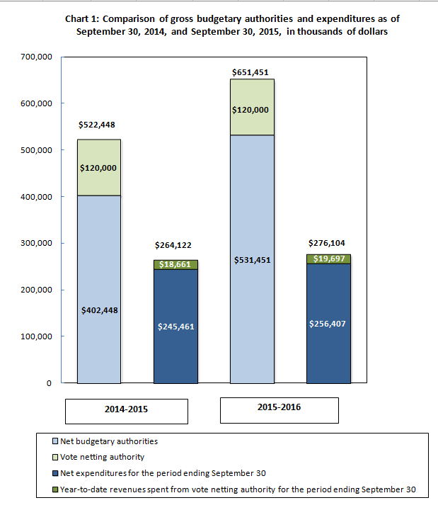
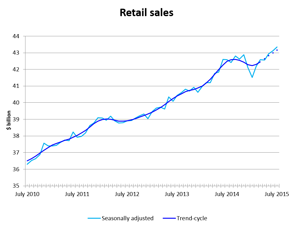
Real-time data tables

New data tables that provide the revision history of 28 economic and social time series are now available. Statistics Canada has always provided its users with the most recent data available, but after consulting some of its expert data users, the agency identified a need for real-time data—or vintage data—to make certain types of analysis easier. These new tables were created to fill this data gap.

Initially, the tables will contain vintages of data as of January 2015. However, some may be expanded to provide users with a longer time series. The real-time table will be released approximately one week after the standard data table.

Background

Statistical revisions are carried out regularly in the compilation of economic and social statistics. These revisions incorporate the most complete and current information from many sources (including surveys, administrative data and public accounts) and use improved estimation methods. While the majority of revisions are done within the months or quarters of a given reference year or on an annual basis, going back two to three years to incorporate benchmark information, some revisions are carried back further to incorporate major changes to concepts or classifications.

Statistics Canada's economic and social statistics programs have well-established policies that govern revisions. Every time Statistics Canada revises data for a given time period, it replaces the existing data table information with the revised data. This ensures that users always have the most up-to-date statistics.

This up-to-date (or revised) information meets the data requirements of most users. However, some users have said that they would like Statistics Canada to provide access to the different vintages of a given time series of economic or social data within a single table or database. A table or database that contains vintages of data is referred to in the international community as a real-time database.

Real-time databases allow users to examine a given time series of economic or social data as it appeared (and was used) at a given point in time before it was revised. This is helpful to users who may want to examine a policy decision—such as a change in interest rates or tax policy—based on the information that was available to policy makers at the time of the decision. These real-time tables help economic and social statistics users to better analyze the impact and development of policy, to prepare forecasts, and to test econometric models.

The revisions in the real-time data tables are not corrections to errors. They represent a normal step in the statistical process, in which statistical agencies produce new vintages of higher quality data as new information becomes available.

Publishing real-time data tables reflects Statistics Canada's values of transparency, accessibility, interpretability, and increased data relevance for users.

Real-time data tables

Statistics Canada will release real-time data for 21 economic and social time series (Table 1).
The real-time data tables will not replace the current data tables for these time series; they are a new product for data users.

The real-time data tables for these economic and social time series will be released approximately one week after the corresponding standard tables have been released and will have their own reference number. At this point, the tables will contain vintages of data starting with the January 2015 reference period. At a later date, some programs may include earlier reference periods to provide users with a longer time series.

Table 1: Real-time data tables
  Regular data table Real-time data table
Historical (real-time) releases of merchandise imports and exports, customs and balance of payments basis for all countries, by seasonal adjustment and North American Product Classification System (NAPCS) 12-10-0163 12-10-0165
Historical (real-time) releases of monthly retail trade, sales 20-10-0056 20-10-0081
Historical (real-time) releases of monthly retail sales, price, and volume 20-10-0067 20-10-0082
Historical (real-time) releases of Consumer Price Index (CPI) statistics, measures of core inflation - Bank of Canada definitions, monthly (percent) 18-10-0256 18-10-0259
Historical (real-time) releases of wholesale trade, sales 20-10-0074 20-10-0019
Historical (real-time) releases of wholesale trade, inventories 20-10-0076 20-10-0020
Historical (real-time) releases of manufacturing sales, by North American Industry Classification System (NAICS) and province 16-10-0048 16-10-0119
Historical (real-time) releases of balance of international payments, current account, seasonally adjusted, quarterly 36-10-0018 36-10-0042
Historical (real-time) releases of gross domestic product (GDP) at basic prices, by industry, monthly 36-10-0434 36-10-0491
Vintages of releases of gross domestic product, income-based 36-10-0103 36-10-0430
Vintages of releases of gross domestic product, expenditure-based 36-10-0104 36-10-0431
Historical (real-time) releases of employment and average weekly earnings (including overtime) for all employees by industry, monthly, seasonally adjusted 14-10-0220 14-10-0331
Historical (real-time) releases of employment and average weekly earnings (including overtime) for all employees by province and territory, monthly, seasonally adjusted 14-10-0223 14-10-0332
Historical (real-time) releases of manufacturers' sales, inventories, orders and inventory to sales ratios, by North American Industry Classification System (NAICS), Canada 16-10-0047 16-10-0118
Historical (real-time) releases of real manufacturing sales, orders, inventory owned and inventory to sales ratio, 2012 dollars, seasonally adjusted 16-10-0013 16-10-0014
Historical (real-time) releases manufacturing capacity utilization rates 16-10-0012 16-10-0015
Historical (real-time) releases of wholesale sales, price and volume, seasonally adjusted 20-10-0003 20-10-0005
Historical (real time) releases of capital and repair expenditures, non-residential tangible assets, by industry and geography 34-10-0035 34-10-0278
Historical (real time) releases of capital and repair expenditures, non-residential tangible assets, by industry, Canada 34-10-0036 34-10-0279

Structure of the real-time tables

The real-time data tables show all revisions of a specific data point over time. Typically, Statistics Canada releases initial estimates for a given period (month or quarter), revises them in subsequent periods based on new information, then revises them again in an annual or historical revision process. Statistics Canada has determined that the most transparent way to present the vintages is to record the date that the data were released in The Daily, the agency's official release vehicle. The real-time data tables are as easy to use as standard tables, but with one important exception: they contain a vintage dimension that records the date of official release.

For example, let us suppose that on November 29, 2019, gross domestic product data for the third quarter of 2019 were released for the first time. The vintage (release) dimension would record the date as November 29, 2019. Suppose that on May 29, 2020, gross domestic product data for the first quarter of 2020 were released for the first time, along with a revised estimate for the third and the last quarter of 2019. A second entry would be made in the table for the third and the fourth quarter of 2019, and the vintage (release) dimension would have the value of May 29, 2020. As new vintages are added, the real-time tables will display the revised data for selected reference periods in columns.

Likewise, the initial estimates for each reference period appear as the last (non-missing) figure in each column. The comparison between the initial  and the most recent estimate therefore represents the difference between the first and last rows in the table for a given reference period. For the most recent reference period, the initial estimate and the most recent estimate are the same.

Figure 1 - Gross Domestic Product, Real-time data

Figure 1 - Gross Domestic Product, Real-time data
Description for Figure 1

This is a real-time data table which shows all revisions of a specific data point over time. On the horizontal axis, the columns indicate calendar years. Each year is subdivided into quarters. The rows of the vertical axis indicate the date data was released.

For each column, the last data point contains the initial data released for that year and quarter. Each subsequent cell above contains revised data for that year and quarter, with the revision date indicated in the corresponding vertical axis.

The first row contains the most recent estimate for each reference period in an economic or social time series. This estimate is consistent with the information in the standard data table for that time series.

Figure 2 - Gross Domestic Product, Real-time data, March 01, 2022

Figure 2 - Gross Domestic Product, Real-time data
Description for Figure 2

This is a real-time data table which shows all revisions of a specific data point over time. On the horizontal axis, the columns indicate calendar years. Each year is subdivided into quarters. The rows of the vertical axis indicate the date data was released.

For each column, the last data point contains the initial data released for that year and quarter. Each subsequent cell above contains revised data for that year and quarter, with the revision date indicated in the corresponding vertical axis.

The data in the top row is circled to show all the data released on that date. The data point at the end of the row is the initial release for the quarter indicated, all preceding data points are the most recent revisions to data previously released for past quarters.

The various revisions for a given reference period are shown in the column for that reference period. The release dates associated with each new reference period are on the left-hand side of the table in the vintage dimension.

Figure 3 - Gross Domestic Product, Real-time data, Q3, 2019

Figure 3 - Gross Domestic Product, Real-time data
Description for Figure 3

This is a real-time data table which shows all revisions of a specific data point over time. On the horizontal axis, the columns indicate calendar years. Each year is subdivided into quarters. The rows of the vertical axis indicate the date data was released.

For each column, the last data point contains the initial data released for that year and quarter. Each subsequent cell above contains revised data for that year and quarter, with the revision date indicated in the corresponding vertical axis.

The data in the first column is circled to show all revisions for a specific quarter since its initial release, at the bottom of the column.

The initial estimate for each reference period is the last figure in each column.

Figure 4 - Gross Domestic Product, Real-time data, November 29, 2019 to 2021

Figure 4 - Gross Domestic Product, Real-time data
Description for Figure 4

This is a real-time data table which shows all revisions of a specific data point over time. On the horizontal axis, the columns indicate calendar years. Each year is subdivided into quarters. The rows of the vertical axis indicate the date data was released.

For each column, the last data point contains the initial data released for that year and quarter. Each subsequent cell above contains revised data for that year and quarter, with the revision date indicated in the corresponding vertical axis.

Finally, if users want to examine the time series as it appeared at a specific point in time, they must select the row associated with that date.

Figure 5 - Gross Domestic Product, Real-time data, March 02, 2021

 Figure 5 - Gross Domestic Product, Real-time data
Description for Figure 5

This is a real-time data table which shows all revisions of a specific data point over time. On the horizontal axis, the columns indicate calendar years. Each year is subdivided into quarters. The rows of the vertical axis indicate the date data was released.

For each column, the last data point contains the initial data released for that year and quarter. Each subsequent cell above contains revised data for that year and quarter, with the revision date indicated in the corresponding vertical axis.

In the middle of the table, a row is circled to illustrate how a time series appeared at a specific point in time.

The importance of footnotes and context

Twenty-one real-time tables have been released to the public, and represent the majority of the key economic and social indicators produced by Statistics Canada. In most cases, revisions occur because the first vintages of estimates are based on incomplete information. As more up to date information becomes available, the data are revised. In some cases, revisions occur due to changes in concepts or methods. These types of revisions need to be analyzed differently than revisions made using updated information.

To help users in their analysis, the real-time tables will include detailed footnotes to provide context for the revisions. These footnotes should be used along with the data to understand how to interpret the various vintages. Specifically, users should exercise caution, since not taking the footnotes and other related metadata into consideration when using real-time data could lead to erroneous conclusions.