Introduction

Modgen is a microsimulation model development package developed by and distributed through Statistics Canada. It was designed to ease the creation, maintenance, and documentation of microsimulation models without the need for advanced programming skills as a prerequisite. It accommodates many different model approaches (continuous or discrete time, case-based or time-based, general or specialized, etc.) Modgen also provides a common visual interface for each model that implements useful functionality such as scenario management, parameter input, the display of output tables from a model run, graphical output of individual biographies, and the display of detailed Modgen-generated model documentation.

In this discussion we introduce a simple microsimulation model called RiskPaths that has been implemented using Modgen. We start with a description of its underlying statistical models and then explore follow-up questions, such as what microsimulation can add to the initial statistical analysis and what other benefits microsimulation can bring to the overall analysis. We then demonstrate parts of Modgen's visual interface to examine elements of the RiskPaths model.

RiskPaths can be used as a model to study childlessness and was developed for training purposes. Technically, RiskPaths is a demographic single sex (female only), data-driven, specialized, continuous time, case-based, competing risk cohort model. It is based on a set of piecewise constant hazard regression models.

In essence, RiskPaths allows the comparison of basic demographic behaviour before and after the political and economic transitions experienced by Russia and Bulgaria around 1989. Its parameters were estimated from Russian and Bulgarian data of the Generations and Gender Survey conducted around 2003/04. Russia and Bulgaria comprise interesting study cases since both countries, after the collapse of socialism, underwent the biggest fertility declines ever observed in history during periods of peace. Furthermore, demographic patterns were very similar and stable in socialist times for both countries, which helps to justify the use of single cohorts as a means of comparison (one representing life in socialist times, the other the life of a post-transition cohort). In this way, the model allows us to compare demographic behaviour before and after the transition, as well as between the two countries themselves.

Share this page
Date modified:

Introduction

In this discussion we explore the microsimulation model development package Modgen and the Modgen application RiskPaths from the model developer's point of view. We first introduce the Modgen programming environment, and then discuss basic Modgen language concepts and the RiskPaths code. Modgen requires only moderate programming skills; thus, after some training, it enables social scientists to create their own models without the need for professional programmers. This is possible because Modgen hides underlying mechanisms like event queuing and automatically creates a stand-alone model with a complete visual interface, including scenario management and model documentation (as introduced in the previous chapter). Model developers can therefore concentrate on model specific code: the declaration of parameters, the states defining the simulated actors, and the events changing the states. High efficiency coding extends also to model output. Modgen includes a powerful language to handle continuous time tabulation. These tabulations are created on-the-fly when simulations are run and the programming to generate them usually requires only a few lines of code per table. Modgen also has a built-in mechanism for estimating the Monte Carlo variation for any cell of any table, without requiring any programming by the model developer.

Being a simple model, RiskPaths does not make use of the full range of available Modgen language concepts and capabilities. The discussion in this chapter does not intend to replace existing Modgen documentation, such as the Modgen Developer's Guide, either. But by introducing the main concepts of Modgen programming, we aim to help you get started in Modgen model development and to engage in further exploration.

Share this page
Date modified:

Basic Modgen concepts

Actor: An actor is the entity whose life is simulated in a Modgen model. A model's actor is often a person, although this is not a requirement--other models have been developed that use dwellings or occupations as actors. Nevertheless, in RiskPaths, the actor is a person or more specifically, a female (since it is a model for the study of childlessness)

State: States describe the characteristics of a model's actors. Some states can be continuous, such as age, whereas others are categorical, such as gender. For categorical states, the actual categories or levels are defined via Modgen's classification command.

Overall, there are two major kinds of states in Modgen-simple states and derived states, both of which are used by RiskPaths and both of which are declared within an actor declaration. A simple state is a state whose value can be initialized and changed by the code that a model developer creates. Simple states are changed by explicitly declared events. A derived state, on the other hand, is a state whose value is given as an expression which is normally derived from or based on other states. A derived state's values are automatically maintained by Modgen throughout a simulation run. An additional useful Modgen concept is the self-scheduling derived state. This is a state which changes in a predefined time sequence, such as integer_age, a state in RiskPaths that changes at each birthday.

Event: In Modgen, simulation takes place through the execution of events. Each event consists of two functions: a time function to determine the time of the next occurrence of the event, and an implementation function to determine the consequences when the event happens. RiskPaths has several events, including a mortality event, union formation and dissolution events, and a first pregnancy event.

Parameter: Parameters are used to give model users a degree of control over the simulations they run. The ability to change different hazards or probabilities that affect various aspects of a simulation allows different scenarios to be explored. Parameters can have many dimensions (such as age, gender, and year) and are stored in .dat data files. In RiskPaths, there is one parameter file, Base(RiskPaths).dat, which stores parameters such as death probabilities by age and risks of first pregnancy by age group. More complex models will usually incorporate more than one .dat file.

Table: Modgen has a powerful cross-tabulation facility built in to report aggregated results in the form of tables. There are two central elements of a table declaration-its captured dimensions (defining when an actor enters and leaves a cell) and its analysis dimension (recording what happens while an actor is in that cell). When running simulations, the tabulations to fill a table are created on the fly, thus removing the need to create and write to large temporary interim files for subsequent reporting. Several examples of table declarations are shown later in this document for the RiskPaths model.

Share this page
Date modified:

How to use BioBrowser: The basics

Beginning a BioBrowser session

To begin a BioBrowser session, click the Start button on your toolbar, choose Programs, and then select BioBrowser.

Opening an existing database file: The File / Open Database command

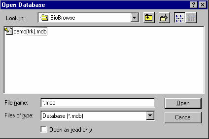
BioBrowser automatically invokes this command at the start of every session. A database file (created by Modgen) must be open before any graphical representations (saved as a biography) can be created.  Although only one database file can be open at a time, any number of biographies can be viewed simultaneously.

A sample database demo(trk).mdb has been supplied as part of the BioBrowser installation.

Dialog box to open demo(trk).mdb database file

Opening a saved biography: The File / Open command

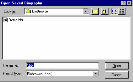
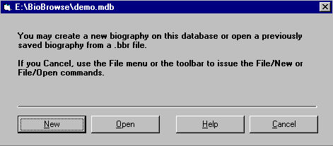
After you have opened the database upon the startup of BioBrowser, you will be asked to either create a new biography or open a saved biography.  One saved biography demo.bbr has been supplied with the installation software.  Choose the Open button.

Information dialog box for opening biography files

You will be prompted for the name of the saved file to open. Choose demo.bbr.

Dialog box to open the saved biography demo.bbr

Creating a new biography: The File / New Biography command

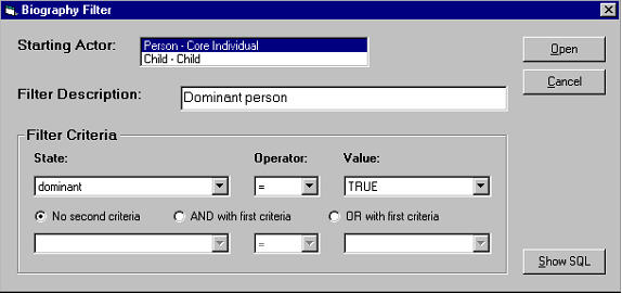
Creating a new biography involves the selection of the actors which you want to graph by choosing a starting actor and a filter.  The way in which the open database was defined in the Modgen model will limit the available choices.  The Starting actor is the type of actor whose state characteristics will be graphed.  Other actors who are linked to these starting actors (e.g.parents, spouses or children) may be added later in the BioBrowser process.  In our example, two starting actors are available: (i) persons, whose states are included in the database only if they are dominant actors or other married or remarried individuals, and (ii) children.

This choice of starting actor may give a large set of actors to be graphed, depending on the size of the Modgen database.  The filter criteria enables you to narrow the focus of the biography. Select a state, an operator on that state, and a value.  This generates a SQL query on the database.  The result of the query is a set of actors which satisfy the filter criteria.  At present, two states can be used to determine the filter.  When selecting two states, you must choose if the criteria will be joined with an “And” or an “Or” condition. If the result of the query is non-empty, then a new biography is opened. Once the biography is open, you may change the criteria using menu item Filter/Criteria…, as discussed in Changing the Biography Filter.

The tracking state is a variable which indicates the ranges of time in which the actors and their states are included in the database.  If you wish to browse all the starting actors, set the filter to Tracking = TRUE in the Filter Criteria section of the Biography Filter dialog box.. 

In the “Filter Description”box you may change the textual description of the filter you have chosen.  It will appear on the bottom of the BioBrowser screen.

In the example below, all person actors whose dominant state is True were selected for browsing. This is a logical state whose value is either True or False for the actor’s lifetime. Since the demo(trk).mdb file was created with only 20 cases, all 20 actors will meet this criteria.

Biography Filter

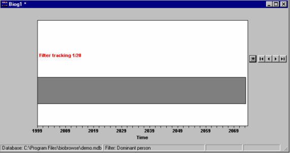
The new biography contains only one display band, the navigation band for the filter tracking state.  It indicates the dates in which the actor’s state characteristics were captured by the model (the axis at the bottom of the screen indicates the start and end dates).  The display band does not have to be continuous.  On the top of this display band the number of actors which satisfied the filter criteria is displayed as well as which actor is presently being shown on the screen.  In the example below, the first actor out of the twenty which were filtered is being displayed. The section State Selection and Navigation explains how more states can be added to the biography.

Sample biography display screen

Saving a biography: The File / Save and File / Save As... commands

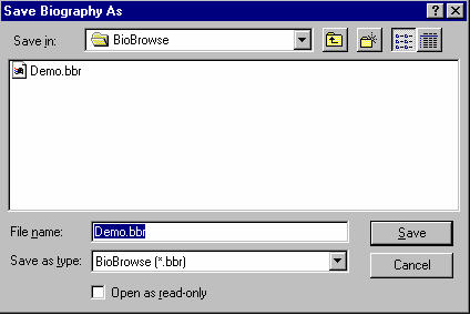
Once all desired states have been added (formatted for style and colour), you may optionally save the biography to file. These files have extension .bbr and may be retrieved at a later time against a compatible data base.  For compatibility, the filter query must be non-empty and all previously selected actor/state pairs must exist in the open database. All style, colour and navigation positions are saved.

Dialog box to save a biography file

If you have altered the state data within a biography, the window caption will display an asterisk (*) after the file name until you save the biography.  This visual asterisk cue is not set, however, by navigation or by changes to global biography options.

Share this page
Date modified:

Microsimulation approaches

PDF Version (PDF, 62.63 KB)

Introduction

This document provides a breakdown of contrasting microsimulation approaches that come into play when we simulate societies with a computer. These approaches can in turn be broken down into approaches of purpose, scope, and methods on how populations are simulated.

With respect to purpose, we mainly distinguish between prediction and explanation, which turns out to also be the distinction in purpose between data-driven empirical microsimulation on one hand and agent based simulation on the other. The prediction approach is further subdivided into a discussion of projections versus forecasts.

There are two aspects covered on the scope of a simulation – we first distinguish general models from specialized ones, then population models from cohort models.

Finally, looking at the methods on how we simulate populations, we focus our discussion in three ways. The first is the population type we simulate, thereby enabling us to distinguish both open versus closed population models, as well as cross-sectional versus synthetic starting populations. The second is the time framework used, either discrete or continuous. The third is the order in which lives are simulated, leading to either a case-based or time-based model.

Purposes of microsimulation: explanation versus prediction

Modeling is abstraction, a reduction of complexity by isolating the driving forces of studied phenomena. The quest to find a formula for human behaviour, especially in economics, is so strong that over-simplified assumptions are an often accepted price for the beauty or elegance of models. The notion that beauty lies in simplicity is even found in some agent based models. Epstein draws an especially appealing analogy between agent based simulation and the paintings of French impressionists, one of these paintings (a street scene) being displayed on the cover of 'Generative Social Sciences' (Epstein 2006). Individuals in all their diversity are only sketched by some dots, but looking from some distance, we are able to clearly recognize the scene.

Can statistical and accounting models compete in beauty with the emergence of social phenomena from a set of simple rules? Hardly--they are complex in nature and require multitudes of parameters. While statisticians might still find elegance in regression functions, beauty is hard to maintain when it comes to filing tax returns or claiming pension benefits. Accounting is boring for most of us, and models based on a multitude of statistical equations and accounting rules can quickly become difficult to understand. So how can microsimulation models compensate for their lack in beauty? The answer is simple: usefulness. In essence, a microsimulation model is useful if it has predictive or explanatory power.

In agent based simulation, explanation means generating social phenomena from the bottom up, the generative standard of explanation being epitomized in the slogan: If you didn't grow it, you didn't explain it (which is regarded as a necessary but not sufficient condition for explanation). This slogan expresses the critique of the agent based community on the mainstream economics community, with the latter's focus on equilibriums without paying too much attention to how or if those equilibriums can ever be reached in reality. Again, agent based models follow a bottom-up approach of generating a virtual society. Their starting points are theories of individual behaviour expressed in computer code. The spectrum of how behaviour is modeled thereby ranges from simple rules to a distributed artificial intelligence approach. In the latter case, the simulated actors are 'intelligent' agents. As such, they have receptors; they get input from the environment. They have cognitive abilities, beliefs and intentions. They have goals, develop strategies, and learn from both their own experiences and those of other agents. This type of simulation is currently almost exclusively done for explanatory purposes. The hope is that the phenomena emerging from the actions and interactions of the agents in the simulation have parallels in real societies. In this way, simulation supports the development of theory.

The contrast to explanation lies in detailed prediction, which constitutes the main purpose of data-driven microsimulation. If microsimulation is designed and used operatively for forecasting and policy recommendations, such models "need to be firmly based in an empirical reality and its relations should have been estimated from real data and carefully tested using well-established statistical and econometric methods. In this case the feasibility of an inference to a real world population or economic process is of great importance" (Klevmarken, 1997).

To predict the future state of a system, there is also a distinction to make between projections and forecasts. Projections are 'what if' predictions. Projections are always 'correct', based on the assumptions that are provided (as long as there are no programming errors). Forecasts are attempts to predict the most likely future, and since there can only be one actual future outcome, most forecasts therefore turn out to be false. With forecasts, we are not just simply trying to find out 'what happens if' (as is the case with projections); instead, we aim to determine the most plausible assumptions and scenarios, thus yielding the most plausible resulting forecast. (It should be noted, however, that implausible assumptions are not necessarily without value. Steady-state assumptions are examples of assumptions that are conceptually appealing and therefore very common but usually implausible. Under such assumptions, individuals are aged in an unchanging world with respect to the socioeconomic context such as economic growth and policies, and the individual behaviour is 'frozen' not allowing for cohort or period effects. Since a cross-section of today's population does not result from a steady-state world, the 'freezing' of individual behaviour and the socioeconomic context can help to isolate and study future dynamics and phenomena resulting from past changes, such as population momentum.)

How different is explanation from prediction? Why can't we rephrase the previous slogan to: If you didn't predict it, you didn't explain it ? First, being able to produce good predictions does not necessarily imply a full understanding of the operations underlying the studied processes. We don't need a full theoretical understanding to predict that lightning is followed by thunder or that fertility is higher in certain life course situations than in others. Predictions can be fully based on observed regularities and trends. In fact, theory is often sacrificed in favour of a highly detailed model that offers a good fit to the data. This, of course, is not without danger. If behaviours are not modeled explicitly, then neither are the corresponding assumptions, which can make the models difficult to understand. We can end up with black-box models. On the other hand, agent based models, while capable of 'growing' some social phenomena, do so in a very stylized way. So far, these models have not reached any sufficient predictive power. In the data-driven microsimulation community, agent based models are thus often regarded as toy models.

Whatever the reason for developing a microsimulation model, however, modellers will typically experience one positive side effect from the exercise: the clarification of concepts. By modeling behaviour, a level of precision (eventually transferred into computer code) is required that is not always found in social science which has an abundance of pure descriptive theory. It is safe to say that the process of modeling itself generates new insights into the processes being modeled (e.g. Burch 1999). While some of these benefits can be experienced in all statistical modeling, simulation adds to the potential. By running a simulation model, we always gain insights into both the reality we are trying to simulate plus the operation of our models and the consequences of our modeling assumptions. In this sense, microsimulation models are always explorative tools, whether their main purpose is explanation or prediction. Or to put it differently, microsimulation models provide experimental platforms for societies where the possibility of genuine natural experiments is limited by nature.

General versus specialized models

The development of larger-scale microsimulation models typically requires a considerable initial investment. This is especially true for policy simulations. Even if only interested in the simulation of one specific policy, we have to create a population and model the demographic changes before we can add the economic behaviour and accounting routines necessary for our study. This can create a situation where it becomes more logical to design microsimulation models as 'general purpose' models, thereby attracting potential investors from various fields. A model capable of detailed pension projections might easily be extended to other tax benefit fields. A model including family structures might be extended to simulate informal care. A struggle for survival can even lead to rather exotic applications–for example, one of the largest models, the US CORSIM model, survived difficult financial times by receiving a grant from a dentist's association interested in a projection of future demands for teeth prosthesis!

It is not surprising, therefore, that there is a general tendency to plan and develop microsimulation applications as general, multi-purpose models right from the beginning. In fact, large general models currently exist for many countries, as shown in the following table.

Country table
Country Models
Australia: APPSIM, DYNAMOD
Canada: DYNACAN, LifePaths
France: DESTINIE
Norway: MOSART
Sweden: SESIM, SVERIGE
UK: SAGEMOD
USA: CORSIM

In creating general models, both the control of ambitions and modularity in the design are crucial for success. Only a few of today's large models have actually reached and stayed at their initially planned sizes. Overambitious approaches have had to be corrected by considerable simplifications, as was the case with DYNAMOD which was initially planned as an integrated micro – macro model.

Specialized microsimulation models concentrate on a few specific behaviours and/or population segments. An example is the NCCSU Long-term Care Model (Hancock et al., 2006). This model simulates the incomes and assets of future cohorts of older people and their ability to contribute towards home care fees. It thereby concentrates on the simulation of the means test of long-term care policies, with the results fed into a macro model of future demands and costs.

Historically, it has also been the case that some models which started off as rather specialized models ended up growing to more general ones. This happened with SESIM and LifePaths, both initially developed for the study of student loans. LifePaths is a particularly interesting example as it not only grew to a large general model but also constituted the base, in a stripped-off version, of a separate family of specialized health models (Statistics Canada's Pohem models).

Cohort versus population models

Cohort models are specialized models, as opposed to general ones, since they only simulate one population segment, namely one birth cohort. This is a useful simplification if we are only interested in studying one cohort or comparing two distinct cohorts.

Economic single cohort studies typically investigate lifetime income and the redistributive effects of tax benefit systems over the life course. Examples of this kind of model include the HARDING and LIFEMOD models developed in parallel, the former for Australia, and the latter for Great Britain (Falkingham and Harding 1996). This kind of model typically assumes a steady-state world, i.e., the HARDING cohort is born in 1960 and lives in a world that looks like Australia in 1986.

Population models deal with the entire population and not just specific cohorts. Not surprisingly, several limitations of cohort models are removed when simulating the whole population, including demographic change issues and distributional issues between cohorts (like intergenerational fairness).

Open versus closed population models

On a global scale, the human population is a closed one. Everybody has been born and will eventually die on this planet, has biological parents born on this planet, and interacts with other humans all sharing these same traits. But, when focusing on the population of a specific region or country, this no longer holds true. People migrate between regions, form partnerships with persons originating in other regions, etc. In such cases, we are dealing with open populations. Therefore, in a simulation model in which we are almost never interested in modeling the whole world population, how can we deal with this problem?

The solution usually requires a degree of creativity. For example, when allowing immigration, we will always have the problem to find ways to model a specific country without modeling the rest of the world. With respect to immigration, many approaches have been adopted, ranging from the cloning of existing 'recent immigrants' to sampling from a host population or even from different 'pools' of host populations representing different regions.

Conceptually more demanding is the simulation of partner matching. In microsimulation, the terms closed and open population usually correspond to whether the matching of spouses is restricted to persons within the population (closed) or whether spouses are 'created on demand' (open). When modeling a closed population, we have the problem that we usually simulate only a sample of a population and not the whole population of a country. If our sample is too small, it becomes unlikely that reasonable matches can be found within the simulated sample. This holds especially true if geography is also an important factor in our model. For example, if there are not many individuals representing the population of a small town, then very few of them will find a partner match within a realistic distance.

The main advantages of closed models are that they allow kinship networks to be tracked and that they enforce more consistency (assuming that they have a large enough population to find appropriate matches). Major drawbacks of closed models, however, are the sampling problems and computational demands associated with partner matching. In a starting population derived from a sample, the model may not be balanced with respect to kinship linkages other than spouses, since a person's parents and siblings are not included in the base population if they do not live in the same household (Toder et al. 2000).

The modeling of open populations requires some abstraction. Here, partners are created on demand - with characteristics synthetically generated or sampled from a host population – and are treated more as attributes of a 'dominant' individual than as 'full' individuals. While their life courses (or some aspects of interest for the simulation of the dominant individual) are simulated, they themselves are not accounted for as individuals in aggregated output.

Cross-sectional versus synthetic starting populations

Every microsimulation model has to start somewhere in time, thus creating the need for a starting population. In population models, we can distinguish two main starting population types: cross-sectional and synthetic. In the first case, we read in a starting population from a cross-sectional dataset and then age all individuals from this moment until death (while of course also adding new individuals at birth events). In the second case we follow an approach typically also found in cohort models–all individuals are modeled from their moment of birth onwards.

If we are only interested in the future, why would we want to start with a synthetic population that would also force us to simulate the past? Certainly, starting from a cross-sectional dataset can be simpler. When we start from representative 'real data', we therefore do not have to retrospectively generate a population, implying that we do not need historical data to model past behaviour. Nor do we have to concern ourselves with consistency problems, since simulations starting with synthetic populations typically lack full cross-sectional consistency.

Unfortunately, many microsimulation applications do need at least some biographical information not available in cross-sectional datasets. For example, past employment and contribution histories determine future pensions. As a consequence, some retrospective or historical modeling will typically be required in most microsimulation applications.

One idea to avoid a synthetic starting population when historical simulation is in fact needed could be to start from an old survey. This idea was followed in the CORSIM model which used a starting population from a 1960 survey (which also makes this model an interesting subject of study itself). While the ensuing possibility to create retrospective forecasts can help assess the model's quality against reality, such an approach nevertheless has its own problems. CORSIM makes heavy use of alignment techniques to recalibrate its retrospective forecasts to published data. Even if many group and aggregate outcomes can be exactly aligned to recent data, there is no way of assuring that the joint distributions based on the 1960 data remain accurate after several decades.

When creating a synthetic starting population, everything is imputed. We thus need models of individual behaviour going back a full century. While such an approach is demanding, it has its advantages. First, the population size is not limited by a survey; we are able to create larger populations, thus diminishing Monte Carlo variability. Second, being created synthetically, we omit confidentiality conflicts. (Statistics Canada follows this approach in its LifePaths model.) Overall, the more that past information has to be imputed, or the more crucial that past information is for what the application is attempting to predict or explain, then the more the approach of a synthetic starting population becomes attractive. For example, Wachter (Wachter 1995) simulated the kinship patterns of the US population following a synthetic starting population approach that went back to the early 19th century. Such detailed kinship information is not found in any survey and thus can be constructed only by means of microsimulation.

Continuous versus discrete time

Models can be distinguished by their time framework which can be either continuous or discrete. Continuous time is usually associated with statistical models of durations to an event, following a competing risk approach. Beginning at a fixed starting point, a random process generates the durations to all considered events, with the event occurring closest to the starting point being the one that is executed while all others are censored. The whole procedure is then repeated at this new starting point in time, and this cycle keep on occurring until the 'death' event of the simulated individual takes place.

Figure 1 illustrates the evolution of a simulated life course in a continuous time model. At the beginning, there are three events (E1, E2, E3), each of which has a randomly generated duration. In the example, E1 occurs first so it becomes the event that is executed; after that, durations for the three events are 're-determined'. However, because E3 is not defined to be contingent on E1 in the example, its duration remains unchanged, whereas new durations are re-generated for E1 and E2. E3 ends up having the next smallest duration so it is executed next.  The cycle then continues as durations are again re-generated for all three events.

Figure 1: Evolution of a simulated life course

Continuous time models are technically very convenient, as they allow new processes to be added without changing the models of the existing processes as long as the statistical requirements for competing risk models are met (See Galler 1997 for a description of associated problems).

Modeling in continuous time, however, does not automatically imply that there are no discrete time (clock) events. Discrete time events can occur when time-dependent covariates are introduced, such as periodically updated economic indices (e.g. unemployment) or flow variables (e.g. personal income). The periodic update of indices then censors all other processes at every periodic time step. If the interruption periods are so short (e.g. one day) that the maximum number of other events within a period virtually becomes one, such a model has converged towards a discrete time model.

Discrete time models determine the states and transitions for every time period while disregarding the exact points of time within the interval. Events are assumed to happen just once in a time period. As several events can take place within one discrete time period, either short periods have to be used to avoid the occurrence of multiple events or else all possible combinations of single events have to be modeled as events themselves. Discrete time frameworks are used in most dynamic tax benefit models, with the older models usually using a yearly time framework mainly due to computational restrictions. With computer power becoming stronger and cheaper over time, however, shorter time steps can be expected to become predominant in future models. When time steps become so short that we can virtually exclude the possibility of multiple events, we have reached 'pseudo-continuity'. In this case we can even use statistical duration models. An example of the combination of both approaches is the Australian DYNAMOD model.

Case-based versus time-based models

The distinction between case-based and time-based models lies in the order in which individual lives are simulated. In case-based models one case is simulated from birth to death before the simulation of the next case begins. Cases can be individual persons or a person plus all 'non-dominant' persons that have been created on demand for this person. In the latter situation, all lives pertaining to a given case are simulated simultaneously over time.

Case-based modeling is only possible if there is no interaction between cases. Interactions are limited to the persons belonging to a case, thereby imposing significant restrictions on what can be modeled. The advantage of such models is of a technical nature--because each case is simulated independently of the others, it is easier to distribute the overall simulation job to several computers. Furthermore, memory can be freed after each case has been simulated, since the underlying information does not have to be stored for future use. (Case-based models can also only be used with open population models, not closed ones).

In time-base models, all individuals are simulated simultaneously over a pre-defined time period. Because all individuals are aging simultaneously (as opposed to just the individuals in one case), the computational demands definitely increase. In a continuous time framework, the next event that happens is the first event scheduled within the entire population. Thus, computer power can still be a bottleneck for this kind of simulation – current models in use typically have population sizes of less than one million.
Share this page
Date modified:

RiskPaths: The underlying statistical models

General description
Events and parameter estimates

General description

Being a model for the study of childlessness, the main event of RiskPaths is the first pregnancy (which is always assumed to lead to birth). Pregnancy can occur at any point in time after the 15th birthday, with risks changing by both age and union status. The underlying statistical models are piecewise constant hazard regressions. With respect to fertility this implies the assumption of a constant pregnancy risk for a given age group (e.g. age 15-17.5) and union status (e.g. single with no prior unions).

For unions, we distinguish four possible state levels:

  • single
  • the first three years in a first union
  • the following years in a first union
  • all the years in a second union

(After the dissolution of a second union, women are assumed to stay single). Accordingly, we model five different union events:

  • first union formation
  • first union dissolution
  • second union formation
  • second union dissolution
  • the change of union phase which occurs after three years in the first union.

The last event (change of union phase) is a clock event - it differs from other events in that its timing is not stochastic but predefined. (Another clock event in the model is the change of the age index every 2.5 years) Besides unions and fertility, we model mortality--a woman may die at any point in time. We stop the simulation of the pregnancy and union events either when a women dies, or at pregnancy (as we are only interested in studying childlessness), or at her 40th birthday (since later first pregnancies are very rare in Russia and Bulgaria and are thus ignored for this model).

At age fifteen a woman becomes subject to both pregnancy and union formation risks. These are competing risks. We draw random durations to first pregnancy and to first union formation. There are two additional competing events at this stage-mortality and change of age group. (As we assume that both pregnancy and union formation risks change with age, the risks underlying the random durations only apply for a given time period--2.5 years in our model--and have to be recalculated at that point in time.)

In other words, the 15th birthday will be followed by one of these four possible events:

  • the woman dies
  • she gets pregnant
  • she enters a union
  • she enters a new age group at age 17.5 because none of the first three events occurred before age 17.5

Death or pregnancy terminates the simulation. A change of age index requires that the waiting times for the competing events union formation and pregnancy be updated. The union formation event alters the risk of first pregnancy (making it much higher) and changes the set of competing risks. A woman is then no longer at risk of first union formation but becomes subject to union dissolution risk.

Events and parameter estimates

First pregnancy

As outlined above, first pregnancy is modeled by an age baseline hazard and relative risks dependent on union status and duration. The following Table 1 displays the parameter estimates for Bulgaria and Russia before and after the political and economical transition.

Table 1
  Bulgaria Russia
15-17.5 0.2869 0.2120
17.5-20 0.7591 0.7606
20-22.5 0.8458 0.8295
22.5-25 0.8167 0.6505
25-27.5 0.6727 0.5423
27.5-30 0.5105 0.5787
30-32.5 0.4882 0.4884
32.5-35 0.2562 0.3237
35-37.5 0.2597 0.3089
37.5-40 0.1542 0.0909
Table 1 before and after the political and economical transition
  before 1989 transition 10 years after transition: 1999+
Bulgaria Russia Bulgaria Russia
Not in union 0.0648 0.0893 0.0316 0.0664
First 3 years of first union 1.0000 1.0000 0.4890 0.5067
First union after three years 0.2523 0.2767 0.2652 0.2746
Second union 0.8048 0.5250 0.2285 0.2698

The data from Table 1 is interpreted as follows in the model. As long as a woman has not entered a partnership, we have to multiply her age-dependent baseline risk of first pregnancy by the relative risk "not in a union". For example, the pregnancy risk of a 20 year old single woman of the pre-transition Bulgarian cohort can be calculated as 0.8458*0.0648 = 0.05481. At this rate of ? =0.05481:

  • The expected mean waiting time to the pregnancy event is 1/ ? = 1/0.05481 = 18.25 years;
  • The probability that a women does not experience pregnancy in the following 2.5 years (given that she stays single) is exp(-?t) = exp(-0.05481*2.5) = 87.2%.

Thus at her 20th birthday, we can draw a random duration to first pregnancy from a uniform distributed random number (a number that can obtain any value between 0 and 1 with the same probability) using the formula:

RandomDuration = -ln(RandomUniform) / (;

As we have calculated above, in 87.2% of the cases, no conception will take place in the next 2.5 years. Accordingly, if we draw a uniform distributed random number smaller than 0.872, the corresponding waiting time will be longer than 2.5 years, since
-ln(RandomUniform) / ( = -ln(0.872)/0.05481 = 2.5 years. A random draw greater than 0.872 will result in a waiting time smaller than 2.5 years-in this situation, if the woman does not enter a union before the pregnancy event, the pregnancy takes place in our simulation.

To continue this example, let us assume that the first event that happens in our simulation is a union formation at age 20.5. We now have to update the pregnancy risk. While the baseline risk still stays the same for the next two years (i.e. 0.8458), the relative risk is now 1.0000 (as per the reference category in Table 1) because the woman is in the first three years of a union. The new hazard rate for pregnancy (applicable for the next two years, until age 22.5) is considerably higher now at 0.8458*1.0000 = 0.8458. The average waiting time at this rate is thus only 1/0.8458 = 1.18 years and for any random number greater than exp(-0.8458*2)=0.1842 the simulated waiting time would be smaller than two years. That is, 81.6% (1 - 0.1842) of women will experience a first pregnancy within the first two years of a first union or partnership that begins at age 20.5.

First union formation

Risks are given as piecewise constant rates changing with age. Again we model age intervals of 2.5 years. These are the rates for women prior to any conception, as such an event would stop our simulation.

Table first union formation
  before 1989 transition 10 years after transition: 1999+
Bulgaria Russia Bulgaria Russia
15-17.5 0.0309 0.0297 0.0173 0.0303
17.5-20 0.1341 0.1342 0.0751 0.1369
20-22.5 0.1672 0.1889 0.0936 0.1926
22.5-25 0.1656 0.1724 0.0927 0.1758
25-27.5 0.1474 0.1208 0.0825 0.1232
27.5-30 0.1085 0.1086 0.0607 0.1108
30-32.5 0.0804 0.0838 0.0450 0.0855
32.5-35 0.0339 0.0862 0.0190 0.0879
35-37.5 0.0455 0.0388 0.0255 0.0396
37.5-40 0.0400 0.0324 0.0224 0.0330

The parameterization example given in Table 2 has the following interpretation: the first union formation hazard of Bulgarian women of the first cohort is 0 until the 15th birthday; afterwards it changes in time steps of 2.5 years from 0.0309 to 0.1341, then from 0.1341 to 0.1672, and so on. The risk is highest for the age group 20-22.5--at a rate of 0.1672, the expected time to union formation is 1/0.1672=6 years. A women who is single on her 20th birthday has a 34% probability of experiencing a first union formation in the following 2.5 years (p=1-exp(-0.1672*2.5)).

Second union formation

A woman becomes exposed to the second union formation risk if and when her first union dissolves. As a difference to the first union formation which is based on age, this process does not start at a fixed point in time but is triggered by another event (first union dissolution). Accordingly, the time intervals of the estimated piecewise constant hazard rates refer to the time since first union dissolution.

Table second union formation
  before 1989 transition 10 years after transition: 1999+
Bulgaria Russia Bulgaria Russia
<2 years after dissolution 0.1996 0.2554 0.1457 0.2247
2-6 years after dissolution 0.1353 0.1695 0.0988 0.1492
6-10 years after dissolution 0.1099 0.1354 0.0802 0.1191
10-15 years after dissolution 0.0261 0.1126 0.0191 0.0991
>5 years after dissolution 0.0457 0.0217 0.0334 0.0191

Union dissolution

Both first and second unions can dissolve, with such processes starting at the first and second union formations, respectively. As the sample size is very small for the modeling of the second union dissolution event we do not distinguish the before and after transition cohorts for this event.

 
  before 1989 transition 10 years after transition: 1999+
Bulgaria Russia Bulgaria Russia
First year of union 0.0096 0.0380 0.0121 0.0601
Union duration 1-5 0.0200 0.0601 0.0252 0.0949
Union duration 5-9 0.0213 0.0476 0.0269 0.0752
Union duration 9-13 0.0151 0.0408 0.0190 0.0645
Union duration >13 0.0111 0.0282 0.0140 0.0445


  Bulgaria Russia
First 3 years of union 0.0371 0.0810
Union duration 3-9 0.0128 0.0744
Union duration 9+ 0.0661 0.0632

Mortality

In this sample model, we leave it to the model user to either set death probabilities by age or to "switch off" mortality allowing the study of fertility without interference from mortality. In the latter case, all women reach the maximum age of 100 years. If the user chooses to simulate mortality, the specified probabilities are internally converted to piecewise constant hazard rates (based on the formula -ln(1-p) for p<1) so that death can happen at any time in a year. If a probability is set to 1 (as is the case when age=100), immediate death is assumed.

Share this page
Date modified:
Share this page
Date modified:

The Modgen programming environment

When installed on a computer, Modgen integrates itself into the (required) Microsoft Visual Studio C++ environment. The visual components of Modgen are a separate toolbar as well as additional items under the Tools and Help menus of Visual Studio. Modgen also appears as an option in the file dialog box for creating a new project as well as in the dialog box for adding a file to an existing project.

Figure 1 displays a screenshot of the programming interface as it appears after opening the Modgen application 'RiskPaths.sln'. The Modgen toolbar consists of several icons for running Modgen, accessing help, opening the BioBrowser tool, and switching the language (between English and French).

Figure 1: The programming interface

Image of programming interface

Modgen code is organized into several files, each with the file extension .mpp. As can be seen in the Solution Explorer window (Figure 1), RiskPaths consists of eight .mpp files grouped in the "Models (mpp)" folder. These are the essential files of RiskPaths, i.e. the files containing all Modgen code written by the model developer.

When invoking the Modgen tool (which can be accessed from the toolbar, or from the first item under the "Tools" menu), these .mpp files are translated into C++ code. Thus Modgen acts as a pre-compiler, creating one .cpp source code file for each .mpp file and putting the resulting .cpp files in the "C++ Files" folder. The Modgen tool also adds model-independent C++ code components to the "C++ Files" folder; these additional filesFootnote 1 should not be changed by the model developer and are essential in order to use the C++ compiler to build the Modgen application.

The model parameters are contained in one or more .dat files organized in a folder labelled "Scenarios". These files are loaded at runtime and contain the actual values assigned to the parameters.

When running the Modgen tool, Modgen - like the C++ compiler - produces log output that is displayed in the Output window. Any error messages are also displayed in this window, and clicking on a particular error message leads you directly to the corresponding Modgen code that produced the error.

Two steps are required to create a Modgen application from the Visual Studio environment. First, Modgen has to translate the Modgen code in the .mpp files; this is done when invoking the Modgen tool. Second, the resulting C++ application has to be built and started. This can be done in one step by selecting "Start Debugging" in the "Debug" menu or by clicking the corresponding icon on the toolbar.

Notes

Footnotes

Footnote 1

ACTORS.CPP, ACTORS.H, app.ico, model.h, model.RC, PARSE.INF, TABINIT.CPP, TABINT.H.

Return to footnote 1 referrer

Share this page
Date modified: